Data preparation
We just use the dataset which are from this step.
library(tidymass)
#> Registered S3 method overwritten by 'Hmisc':
#>   method       from
#>   vcov.default fit.models
#> ── Attaching packages ────────────────────────────── tidymass 1.0.9 ──
#> ✔ massdataset   1.0.34     ✔ metid         1.2.33
#> ✔ massprocesser 1.0.10     ✔ masstools     1.0.13
#> ✔ masscleaner   1.0.12     ✔ dplyr         1.1.4
#> ✔ massqc        1.0.7      ✔ ggplot2       3.5.1
#> ✔ massstat      1.0.6      ✔ magrittr      2.0.3
#> ✔ metpath       1.0.8
load("data_cleaning/POS/object_pos")
load("data_cleaning/NEG/object_neg")
Change batch to character.
object_pos <-
  object_pos %>%
  activate_mass_dataset(what = "sample_info") %>%
  dplyr::mutate(batch = as.character(batch))

object_neg <-
  object_neg %>%
  activate_mass_dataset(what = "sample_info") %>%
  dplyr::mutate(batch = as.character(batch))
object_pos
#> --------------------
#> massdataset version: 0.99.8
#> --------------------
#> 1.expression_data:[ 10149 x 259 data.frame]
#> 2.sample_info:[ 259 x 6 data.frame]
#> 259 samples:sample_06 sample_103 sample_11 ... sample_QC_38 sample_QC_39
#> 3.variable_info:[ 10149 x 3 data.frame]
#> 10149 variables:M70T73_POS M70T53_POS M70T183_POS ... M923T55_POS M992T641_POS
#> 4.sample_info_note:[ 6 x 2 data.frame]
#> 5.variable_info_note:[ 3 x 2 data.frame]
#> 6.ms2_data:[ 0 variables x 0 MS2 spectra]
#> --------------------
#> Processing information
#> 3 processings in total
#> create_mass_dataset ----------
#>       Package         Function.used                Time
#> 1 massdataset create_mass_dataset() 2022-02-23 08:37:06
#> process_data ----------
#>         Package Function.used                Time
#> 1 massprocesser  process_data 2022-02-23 08:36:42
#> mutate ----------
#>       Package Function.used                Time
#> 1 massdataset      mutate() 2024-09-25 19:53:23
object_neg
#> --------------------
#> massdataset version: 0.99.8
#> --------------------
#> 1.expression_data:[ 8804 x 259 data.frame]
#> 2.sample_info:[ 259 x 6 data.frame]
#> 259 samples:sample_06 sample_103 sample_11 ... sample_QC_38 sample_QC_39
#> 3.variable_info:[ 8804 x 3 data.frame]
#> 8804 variables:M70T712_NEG M70T527_NEG M70T587_NEG ... M941T65_NEG M948T641_NEG
#> 4.sample_info_note:[ 6 x 2 data.frame]
#> 5.variable_info_note:[ 3 x 2 data.frame]
#> 6.ms2_data:[ 0 variables x 0 MS2 spectra]
#> --------------------
#> Processing information
#> 3 processings in total
#> create_mass_dataset ----------
#>       Package         Function.used                Time
#> 1 massdataset create_mass_dataset() 2022-02-23 08:38:19
#> process_data ----------
#>         Package Function.used                Time
#> 1 massprocesser  process_data 2022-02-23 08:38:02
#> mutate ----------
#>       Package Function.used                Time
#> 1 massdataset      mutate() 2024-09-25 19:53:23
Data quality assessment before data cleaning
Here, we can use the massqc package to assess the data quality.
We can just use the massqc_report() function to get a html format quality assessment report.
massqc::massqc_report(object = object_pos,
                      path = "data_cleaning/POS/data_quality_before_data_cleaning")
A html format report and pdf figures will be placed in the folder data_cleaning/POS/data_quality_before_data_cleaning/Report.

The html report is below:
Negative mode.
massqc::massqc_report(object = object_neg,
                      path = "data_cleaning/NEG/data_quality_before_data_cleaning")
The PCA score plot is used to show the batch effect of positive and negative dataset.
Positive mode:
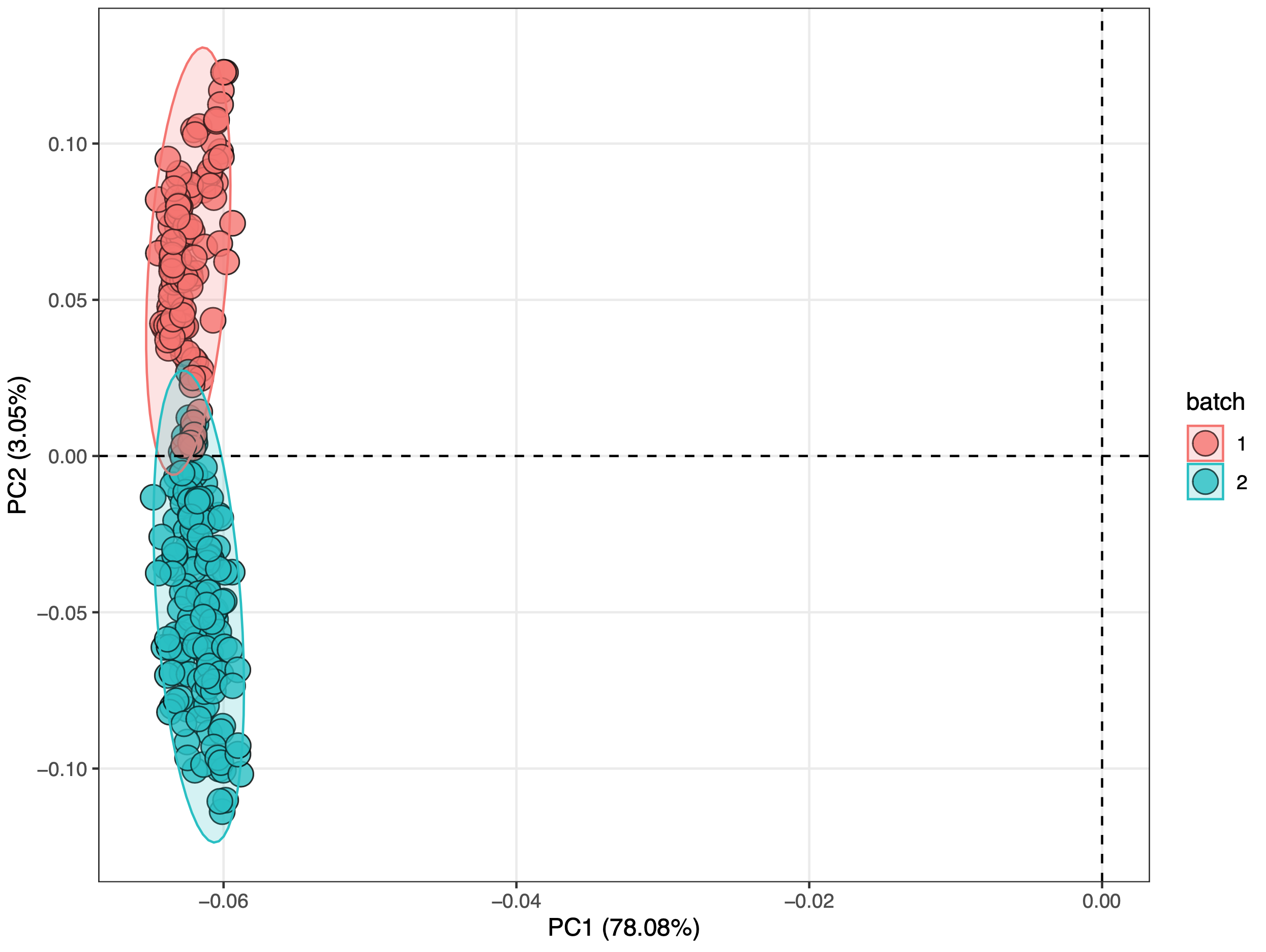
We can see that no matter in positive and negative mode, batch effect is serious.
Remove noisy metabolic features
Remove variables which have MVs in more than 20% QC samples and in at lest 50% samples in control group or case group.
Positive mode
object_pos %>%
  activate_mass_dataset(what = "sample_info") %>%
  dplyr::count(group)
#>     group   n
#> 1    Case 110
#> 2 Control 110
#> 3      QC  39
MV percentage in QC samples.
show_variable_missing_values(object = object_pos %>%
                               activate_mass_dataset(what = "sample_info") %>%
                               filter(class == "QC"),
                             percentage = TRUE) +
  scale_size_continuous(range = c(0.01, 2))

qc_id =
  object_pos %>%
  activate_mass_dataset(what = "sample_info") %>%
  filter(class == "QC") %>%
  pull(sample_id)

control_id =
  object_pos %>%
  activate_mass_dataset(what = "sample_info") %>%
  filter(group == "Control") %>%
  pull(sample_id)

case_id =
  object_pos %>%
  activate_mass_dataset(what = "sample_info") %>%
  filter(group == "Case") %>%
  pull(sample_id)

object_pos =
  object_pos %>%
  mutate_variable_na_freq(according_to_samples = qc_id) %>%
  mutate_variable_na_freq(according_to_samples = control_id) %>%
  mutate_variable_na_freq(according_to_samples = case_id)

head(extract_variable_info(object_pos))
#>   variable_id       mz        rt    na_freq na_freq.1 na_freq.2
#> 1  M70T73_POS 70.04074  73.31705 0.28205128 0.6000000 0.4727273
#> 2  M70T53_POS 70.06596  52.78542 0.00000000 0.1454545 0.0000000
#> 3 M70T183_POS 70.19977 182.87981 0.00000000 0.6636364 0.7454545
#> 4 M70T527_POS 70.36113 526.76657 0.02564103 0.1818182 0.3000000
#> 5 M71T695_POS 70.56911 694.84592 0.02564103 0.6454545 0.5545455
#> 6 M71T183_POS 70.75034 182.77790 0.05128205 0.7272727 0.7909091
Remove variables.
object_pos <-
  object_pos %>%
  activate_mass_dataset(what = "variable_info") %>%
  filter(na_freq < 0.2 & (na_freq.1 < 0.5 | na_freq.2 < 0.5))
object_pos
#> --------------------
#> massdataset version: 0.99.8
#> --------------------
#> 1.expression_data:[ 5101 x 259 data.frame]
#> 2.sample_info:[ 259 x 6 data.frame]
#> 259 samples:sample_06 sample_103 sample_11 ... sample_QC_38 sample_QC_39
#> 3.variable_info:[ 5101 x 6 data.frame]
#> 5101 variables:M70T53_POS M70T527_POS M71T775_POS ... M836T610_POS M836T759_POS
#> 4.sample_info_note:[ 6 x 2 data.frame]
#> 5.variable_info_note:[ 6 x 2 data.frame]
#> 6.ms2_data:[ 0 variables x 0 MS2 spectra]
#> --------------------
#> Processing information
#> 5 processings in total
#> create_mass_dataset ----------
#>       Package         Function.used                Time
#> 1 massdataset create_mass_dataset() 2022-02-23 08:37:06
#> process_data ----------
#>         Package Function.used                Time
#> 1 massprocesser  process_data 2022-02-23 08:36:42
#> mutate ----------
#>       Package Function.used                Time
#> 1 massdataset      mutate() 2024-09-25 19:53:23
#> mutate_variable_na_freq ----------
#>       Package             Function.used                       Time
#> 1 massdataset mutate_variable_na_freq() 2024-09-25 19:53:25.443142
#> 2 massdataset mutate_variable_na_freq() 2024-09-25 19:53:25.465639
#> 3 massdataset mutate_variable_na_freq() 2024-09-25 19:53:25.505201
#> filter ----------
#>       Package Function.used                Time
#> 1 massdataset      filter() 2024-09-25 19:53:25
Only 5,101 variables left.
Negative mode
object_neg %>%
  activate_mass_dataset(what = "sample_info") %>%
  dplyr::count(group)
#>     group   n
#> 1    Case 110
#> 2 Control 110
#> 3      QC  39
MV percentage in QC samples.
show_variable_missing_values(object = object_neg %>%
                               activate_mass_dataset(what = "sample_info") %>%
                               filter(class == "QC"),
                             percentage = TRUE) +
  scale_size_continuous(range = c(0.01, 2))

qc_id =
  object_neg %>%
  activate_mass_dataset(what = "sample_info") %>%
  filter(class == "QC") %>%
  pull(sample_id)

control_id =
  object_neg %>%
  activate_mass_dataset(what = "sample_info") %>%
  filter(group == "Control") %>%
  pull(sample_id)

case_id =
  object_neg %>%
  activate_mass_dataset(what = "sample_info") %>%
  filter(group == "Case") %>%
  pull(sample_id)

object_neg =
  object_neg %>%
  mutate_variable_na_freq(according_to_samples = qc_id) %>%
  mutate_variable_na_freq(according_to_samples = control_id) %>%
  mutate_variable_na_freq(according_to_samples = case_id)

head(extract_variable_info(object_neg))
#>   variable_id       mz        rt    na_freq   na_freq.1   na_freq.2
#> 1 M70T712_NEG 70.05911 711.97894 0.05128205 0.109090909 0.018181818
#> 2 M70T527_NEG 70.13902 526.85416 0.33333333 0.509090909 0.618181818
#> 3 M70T587_NEG 70.31217 587.25330 0.00000000 0.009090909 0.009090909
#> 4  M70T47_NEG 70.33835  46.57537 0.84615385 0.936363636 0.090909091
#> 5 M71T587_NEG 70.56315 587.02570 0.17948718 0.145454545 0.163636364
#> 6 M71T641_NEG 70.70657 641.16672 0.10256410 0.063636364 0.072727273
Remove variables.
object_neg <-
  object_neg %>%
  activate_mass_dataset(what = "variable_info") %>%
  filter(na_freq < 0.2 & (na_freq.1 < 0.5 | na_freq.2 < 0.5))
object_neg
#> --------------------
#> massdataset version: 0.99.8
#> --------------------
#> 1.expression_data:[ 4104 x 259 data.frame]
#> 2.sample_info:[ 259 x 6 data.frame]
#> 259 samples:sample_06 sample_103 sample_11 ... sample_QC_38 sample_QC_39
#> 3.variable_info:[ 4104 x 6 data.frame]
#> 4104 variables:M70T712_NEG M70T587_NEG M71T587_NEG ... M884T57_NEG M899T56_NEG
#> 4.sample_info_note:[ 6 x 2 data.frame]
#> 5.variable_info_note:[ 6 x 2 data.frame]
#> 6.ms2_data:[ 0 variables x 0 MS2 spectra]
#> --------------------
#> Processing information
#> 5 processings in total
#> create_mass_dataset ----------
#>       Package         Function.used                Time
#> 1 massdataset create_mass_dataset() 2022-02-23 08:38:19
#> process_data ----------
#>         Package Function.used                Time
#> 1 massprocesser  process_data 2022-02-23 08:38:02
#> mutate ----------
#>       Package Function.used                Time
#> 1 massdataset      mutate() 2024-09-25 19:53:23
#> mutate_variable_na_freq ----------
#>       Package             Function.used                       Time
#> 1 massdataset mutate_variable_na_freq() 2024-09-25 19:53:26.396638
#> 2 massdataset mutate_variable_na_freq() 2024-09-25 19:53:26.426459
#> 3 massdataset mutate_variable_na_freq() 2024-09-25 19:53:26.447222
#> filter ----------
#>       Package Function.used                Time
#> 1 massdataset      filter() 2024-09-25 19:53:26
4104 features left.
Filter outlier samples
We can use the detect_outlier() to find the outlier samples.
More information about how to detect outlier samples can be found here.
Positive mode
massdataset::show_sample_missing_values(object = object_pos,
                                        color_by = "group",
                                        order_by = "injection.order",
                                        percentage = TRUE) +
  theme(axis.text.x = element_text(size = 2)) +
  scale_size_continuous(range = c(0.1, 2)) +
  ggsci::scale_color_aaas()

Detect outlier samples.
outlier_samples =
  object_pos %>%
  `+`(1) %>%
  log(2) %>%
  scale() %>%
  detect_outlier()

outlier_samples
#> --------------------
#> masscleaner
#> --------------------
#> 1 according_to_na : 0 outlier samples.
#> 2 according_to_pc_sd : 0 outlier samples.
#> 3 according_to_pc_mad : 0 outlier samples.
#> 4 accordint_to_distance : 0 outlier samples.
#> extract all outlier table using extract_outlier_table()
outlier_table <-
extract_outlier_table(outlier_samples)

outlier_table %>%
  head()
#>            according_to_na pc_sd pc_mad accordint_to_distance
#> sample_06            FALSE FALSE  FALSE                 FALSE
#> sample_103           FALSE FALSE  FALSE                 FALSE
#> sample_11            FALSE FALSE  FALSE                 FALSE
#> sample_112           FALSE FALSE  FALSE                 FALSE
#> sample_117           FALSE FALSE  FALSE                 FALSE
#> sample_12            FALSE FALSE  FALSE                 FALSE

outlier_table %>%
  apply(1, function(x){
    sum(x)
  }) %>%
  `>`(0) %>%
  which()
#> named integer(0)
No outlier samples in positive mode.
Negative mode
massdataset::show_sample_missing_values(object = object_neg,
                                        color_by = "group",
                                        order_by = "injection.order",
                                        percentage = TRUE) +
  theme(axis.text.x = element_text(size = 2)) +
  scale_size_continuous(range = c(0.1, 2)) +
  ggsci::scale_color_aaas()

Detect outlier samples.
outlier_samples =
  object_neg %>%
  `+`(1) %>%
  log(2) %>%
  scale() %>%
  detect_outlier()

outlier_samples
#> --------------------
#> masscleaner
#> --------------------
#> 1 according_to_na : 0 outlier samples.
#> 2 according_to_pc_sd : 0 outlier samples.
#> 3 according_to_pc_mad : 0 outlier samples.
#> 4 accordint_to_distance : 0 outlier samples.
#> extract all outlier table using extract_outlier_table()
outlier_table <-
extract_outlier_table(outlier_samples)

outlier_table %>%
  head()
#>            according_to_na pc_sd pc_mad accordint_to_distance
#> sample_06            FALSE FALSE  FALSE                 FALSE
#> sample_103           FALSE FALSE  FALSE                 FALSE
#> sample_11            FALSE FALSE  FALSE                 FALSE
#> sample_112           FALSE FALSE  FALSE                 FALSE
#> sample_117           FALSE FALSE  FALSE                 FALSE
#> sample_12            FALSE FALSE  FALSE                 FALSE

outlier_table %>%
  apply(1, function(x){
    sum(x)
  }) %>%
  `>`(0) %>%
  which()
#> named integer(0)
No outlier samples in negative mode.
Missing value imputation
get_mv_number(object_pos)
#> [1] 148965
object_pos <-
  impute_mv(object = object_pos, method = "knn")
#> Cluster size 4983 broken into 88 4895
#> Done cluster 88
#> Cluster size 4895 broken into 4497 398
#> Cluster size 4497 broken into 3737 760
#> Cluster size 3737 broken into 2703 1034
#> Cluster size 2703 broken into 1706 997
#> Cluster size 1706 broken into 1240 466
#> Done cluster 1240
#> Done cluster 466
#> Done cluster 1706
#> Done cluster 997
#> Done cluster 2703
#> Done cluster 1034
#> Done cluster 3737
#> Done cluster 760
#> Done cluster 4497
#> Done cluster 398
#> Done cluster 4895

get_mv_number(object_pos)
#> [1] 0
get_mv_number(object_neg)
#> [1] 146427

object_neg <-
  impute_mv(object = object_neg, method = "knn")
#> Cluster size 4006 broken into 3965 41
#> Cluster size 3965 broken into 3743 222
#> Cluster size 3743 broken into 505 3238
#> Done cluster 505
#> Cluster size 3238 broken into 2519 719
#> Cluster size 2519 broken into 1721 798
#> Cluster size 1721 broken into 676 1045
#> Done cluster 676
#> Done cluster 1045
#> Done cluster 1721
#> Done cluster 798
#> Done cluster 2519
#> Done cluster 719
#> Done cluster 3238
#> Done cluster 3743
#> Done cluster 222
#> Done cluster 3965
#> Done cluster 41

get_mv_number(object_neg)
#> [1] 0
Data normalization and integration
Positive mode
object_pos <-
  normalize_data(object_pos, method = "median")

object_pos2 <-
  integrate_data(object_pos, method = "subject_median")
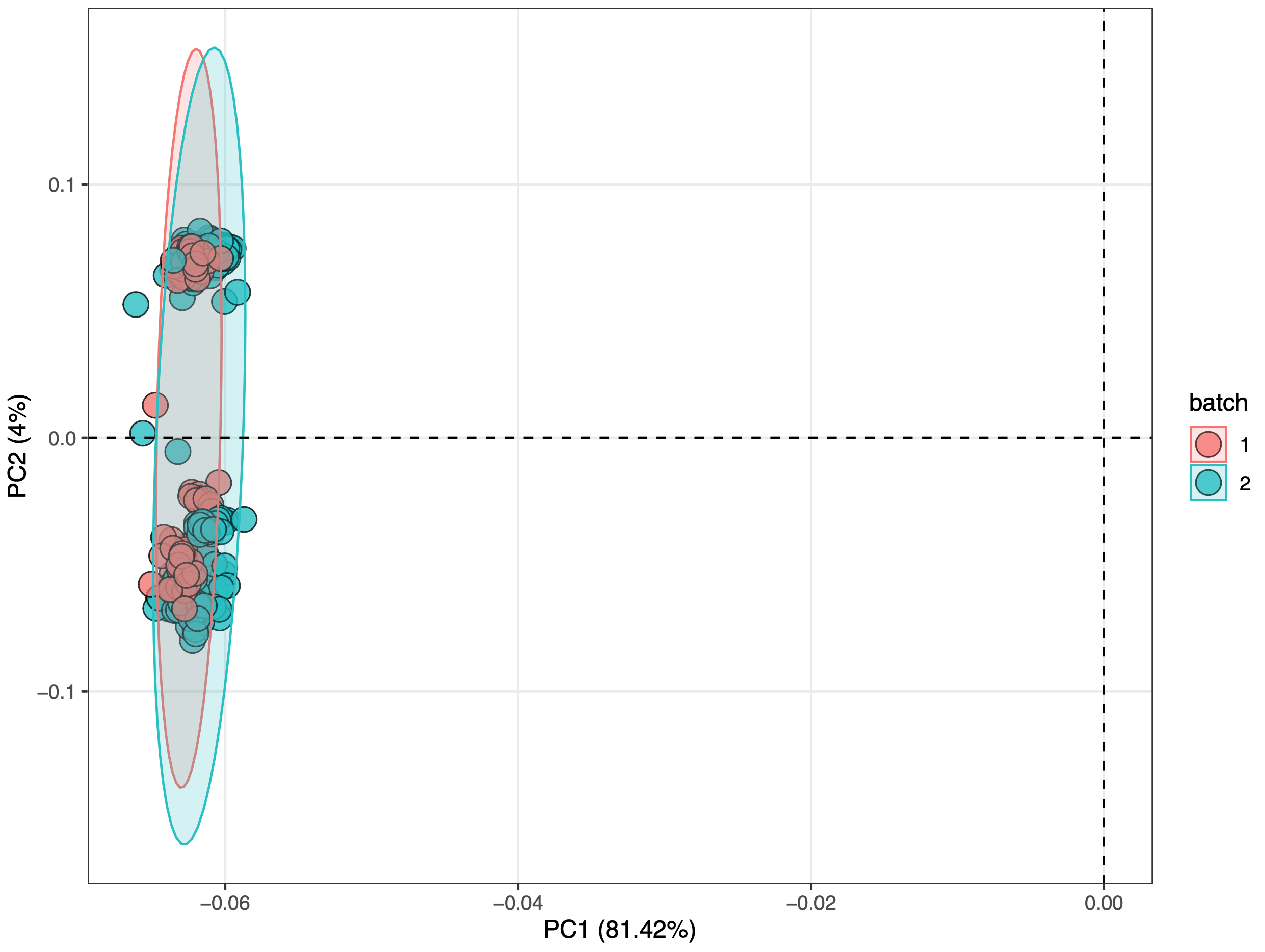
object_pos2 %>%
  `+`(1) %>%
  log(2) %>%
  massqc::massqc_pca(color_by = "batch", line = FALSE)

Negative mode
object_neg <-
  normalize_data(object_neg, method = "median")

object_neg2 <-
  integrate_data(object_neg, method = "subject_median")
object_neg2 %>%
  `+`(1) %>%
  log(2) %>%
  massqc::massqc_pca(color_by = "batch", line = FALSE)

Save data for subsequent analysis.
save(object_pos2, file = "data_cleaning/POS/object_pos2")
save(object_neg2, file = "data_cleaning/NEG/object_neg2")
Session information
sessionInfo()
#> R version 4.4.1 (2024-06-14)
#> Platform: aarch64-apple-darwin20
#> Running under: macOS 15.0
#>
#> Matrix products: default
#> BLAS:   /Library/Frameworks/R.framework/Versions/4.4-arm64/Resources/lib/libRblas.0.dylib
#> LAPACK: /Library/Frameworks/R.framework/Versions/4.4-arm64/Resources/lib/libRlapack.dylib;  LAPACK version 3.12.0
#>
#> locale:
#> [1] en_US.UTF-8/en_US.UTF-8/en_US.UTF-8/C/en_US.UTF-8/en_US.UTF-8
#>
#> time zone: Asia/Singapore
#> tzcode source: internal
#>
#> attached base packages:
#> [1] grid      stats4    stats     graphics  grDevices utils     datasets
#> [8] methods   base
#>
#> other attached packages:
#>  [1] metid_1.2.33          metpath_1.0.8         ComplexHeatmap_2.20.0
#>  [4] mixOmics_6.28.0       lattice_0.22-6        MASS_7.3-61
#>  [7] massstat_1.0.6        tidyr_1.3.1           ggfortify_0.4.17
#> [10] massqc_1.0.7          masscleaner_1.0.12    MSnbase_2.30.1
#> [13] ProtGenerics_1.36.0   S4Vectors_0.42.1      Biobase_2.64.0
#> [16] BiocGenerics_0.50.0   mzR_2.38.0            Rcpp_1.0.13
#> [19] xcms_4.2.3            BiocParallel_1.38.0   massprocesser_1.0.10
#> [22] ggplot2_3.5.1         dplyr_1.1.4           magrittr_2.0.3
#> [25] masstools_1.0.13      massdataset_1.0.34    tidymass_1.0.9
#>
#> loaded via a namespace (and not attached):
#>   [1] fs_1.6.4                    matrixStats_1.3.0
#>   [3] bitops_1.0-8                fit.models_0.64
#>   [5] httr_1.4.7                  RColorBrewer_1.1-3
#>   [7] doParallel_1.0.17           ggsci_3.2.0
#>   [9] tools_4.4.1                 doRNG_1.8.6
#>  [11] backports_1.5.0             utf8_1.2.4
#>  [13] R6_2.5.1                    lazyeval_0.2.2
#>  [15] GetoptLong_1.0.5            withr_3.0.1
#>  [17] prettyunits_1.2.0           gridExtra_2.3
#>  [19] preprocessCore_1.66.0       cli_3.6.3
#>  [21] fastDummies_1.7.4           labeling_0.4.3
#>  [23] sass_0.4.9                  mvtnorm_1.3-1
#>  [25] robustbase_0.99-4           readr_2.1.5
#>  [27] randomForest_4.7-1.1        proxy_0.4-27
#>  [29] pbapply_1.7-2               systemfonts_1.1.0
#>  [31] foreign_0.8-87              svglite_2.1.3
#>  [33] rrcov_1.7-6                 MetaboCoreUtils_1.12.0
#>  [35] parallelly_1.38.0           itertools_0.1-3
#>  [37] limma_3.60.4                readxl_1.4.3
#>  [39] rstudioapi_0.16.0           impute_1.78.0
#>  [41] generics_0.1.3              shape_1.4.6.1
#>  [43] zip_2.3.1                   Matrix_1.7-0
#>  [45] MALDIquant_1.22.3           fansi_1.0.6
#>  [47] abind_1.4-5                 lifecycle_1.0.4
#>  [49] yaml_2.3.10                 SummarizedExperiment_1.34.0
#>  [51] SparseArray_1.4.8           crayon_1.5.3
#>  [53] PSMatch_1.8.0               KEGGREST_1.44.1
#>  [55] pillar_1.9.0                knitr_1.48
#>  [57] GenomicRanges_1.56.1        rjson_0.2.22
#>  [59] corpcor_1.6.10              codetools_0.2-20
#>  [61] glue_1.7.0                  pcaMethods_1.96.0
#>  [63] data.table_1.16.0           remotes_2.5.0
#>  [65] MultiAssayExperiment_1.30.3 vctrs_0.6.5
#>  [67] png_0.1-8                   cellranger_1.1.0
#>  [69] gtable_0.3.5                cachem_1.1.0
#>  [71] xfun_0.47                   openxlsx_4.2.7
#>  [73] S4Arrays_1.4.1              tidygraph_1.3.1
#>  [75] pcaPP_2.0-5                 ncdf4_1.23
#>  [77] iterators_1.0.14            statmod_1.5.0
#>  [79] robust_0.7-5                progress_1.2.3
#>  [81] GenomeInfoDb_1.40.1         rprojroot_2.0.4
#>  [83] bslib_0.8.0                 affyio_1.74.0
#>  [85] rpart_4.1.23                colorspace_2.1-1
#>  [87] DBI_1.2.3                   Hmisc_5.1-3
#>  [89] nnet_7.3-19                 tidyselect_1.2.1
#>  [91] compiler_4.4.1              MassSpecWavelet_1.70.0
#>  [93] htmlTable_2.4.3             DelayedArray_0.30.1
#>  [95] plotly_4.10.4               bookdown_0.40
#>  [97] checkmate_2.3.2             scales_1.3.0
#>  [99] DEoptimR_1.1-3              affy_1.82.0
#> [101] stringr_1.5.1               digest_0.6.37
#> [103] rmarkdown_2.28              XVector_0.44.0
#> [105] htmltools_0.5.8.1           pkgconfig_2.0.3
#> [107] base64enc_0.1-3             MatrixGenerics_1.16.0
#> [109] highr_0.11                  fastmap_1.2.0
#> [111] rlang_1.1.4                 GlobalOptions_0.1.2
#> [113] htmlwidgets_1.6.4           UCSC.utils_1.0.0
#> [115] farver_2.1.2                jquerylib_0.1.4
#> [117] jsonlite_1.8.8              MsExperiment_1.6.0
#> [119] mzID_1.42.0                 RCurl_1.98-1.16
#> [121] Formula_1.2-5               GenomeInfoDbData_1.2.12
#> [123] patchwork_1.2.0             munsell_0.5.1
#> [125] viridis_0.6.5               MsCoreUtils_1.16.1
#> [127] vsn_3.72.0                  furrr_0.3.1
#> [129] stringi_1.8.4               ggraph_2.2.1
#> [131] zlibbioc_1.50.0             plyr_1.8.9
#> [133] parallel_4.4.1              listenv_0.9.1
#> [135] ggrepel_0.9.5               Biostrings_2.72.1
#> [137] MsFeatures_1.12.0           graphlayouts_1.1.1
#> [139] hms_1.1.3                   Spectra_1.14.1
#> [141] circlize_0.4.16             igraph_2.0.3
#> [143] QFeatures_1.14.2            rngtools_1.5.2
#> [145] reshape2_1.4.4              XML_3.99-0.17
#> [147] evaluate_0.24.0             blogdown_1.19
#> [149] BiocManager_1.30.25         tzdb_0.4.0
#> [151] foreach_1.5.2               missForest_1.5
#> [153] tweenr_2.0.3                purrr_1.0.2
#> [155] polyclip_1.10-7             future_1.34.0
#> [157] clue_0.3-65                 ggforce_0.4.2
#> [159] AnnotationFilter_1.28.0     e1071_1.7-14
#> [161] RSpectra_0.16-2             ggcorrplot_0.1.4.1
#> [163] viridisLite_0.4.2           class_7.3-22
#> [165] rARPACK_0.11-0              tibble_3.2.1
#> [167] memoise_2.0.1               ellipse_0.5.0
#> [169] IRanges_2.38.1              cluster_2.1.6
#> [171] globals_0.16.3              here_1.0.1