Introduction to Metabolomics Data
The Danish Project Project studies metabolic changes during human pregnancy and if these altered metabolites could be used to predict preterm.
Referenced research
Introduction to tidyMass project
TidyMass is an ecosystem of R packages that share an underlying design philosophy, grammar, and data structure, which provides a comprehensive, reproducible, and object-oriented computational framework. The modular architecture makes tidyMass a highly flexible and extensible tool, which other users can improve and integrate with other tools to customize their own pipeline.
More information about tidyMass could be found here: tidymass.org.
Hopefully, at the end of this module, you will have a better sense of the metabolomics data analysis procedure and how to use R for reproducible data processing and analysis
Data preparation
Download the demo data and uncompress it.
-
If you can use Google drive, download here. (code 2022)
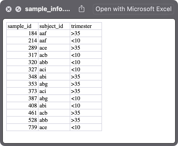
The demo data contains RPLC positive mode, with 7 participants, and two samples for each participant (Trimester 1 (< 10 weeks) and trimester 3 (> 30 weeks)). So there are 14 samples in total.
-
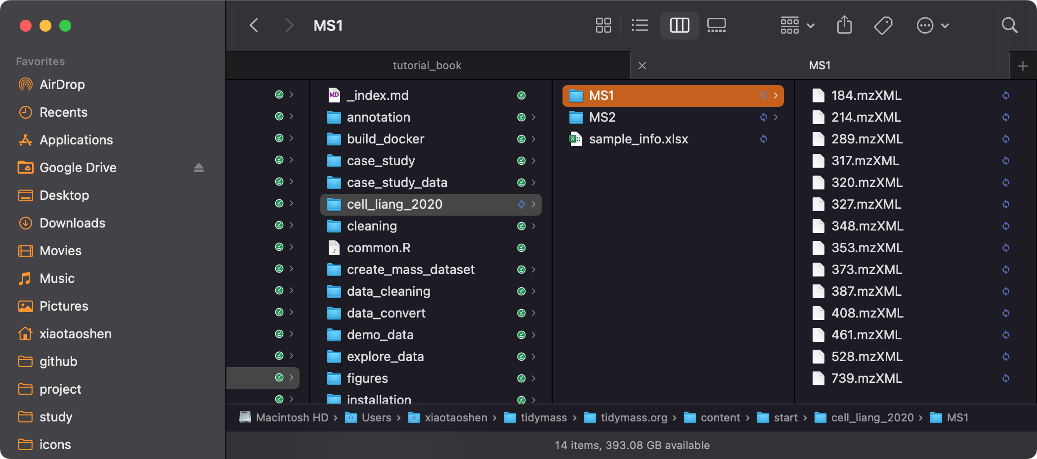
MS1: MS1 is the folder contains the mzXML for 14 samples. -
MS2: MS2 is the folder contains the mgf for QC samples (MS2 spectra). -
sample_info.xlsx: it is the metadata for samples.
Raw data processing
library(tidymass)
#> Registered S3 method overwritten by 'Hmisc':
#>   method       from
#>   vcov.default fit.models
#> ── Attaching packages ──────────────────────────────────────── tidymass 1.0.9 ──
#> ✔ massdataset   1.0.34     ✔ metid         1.2.33
#> ✔ massprocesser 1.0.10     ✔ masstools     1.0.13
#> ✔ masscleaner   1.0.12     ✔ dplyr         1.1.4
#> ✔ massqc        1.0.7      ✔ ggplot2       3.5.1
#> ✔ massstat      1.0.6      ✔ magrittr      2.0.3
#> ✔ metpath       1.0.8
library(tidyverse)
#> ── Attaching core tidyverse packages ──────────────────────── tidyverse 2.0.0 ──
#> ✔ forcats   1.0.0     ✔ readr     2.1.5
#> ✔ lubridate 1.9.3     ✔ stringr   1.5.1
#> ✔ purrr     1.0.2     ✔ tibble    3.2.1
#> ── Conflicts ────────────────────────────────────────── tidyverse_conflicts() ──
#> ✖ xcms::collect()          masks dplyr::collect()
#> ✖ MSnbase::combine()       masks Biobase::combine(), BiocGenerics::combine(), dplyr::combine()
#> ✖ tidyr::expand()          masks S4Vectors::expand()
#> ✖ tidyr::extract()         masks magrittr::extract()
#> ✖ metid::filter()          masks metpath::filter(), dplyr::filter(), massdataset::filter(), stats::filter()
#> ✖ S4Vectors::first()       masks dplyr::first()
#> ✖ xcms::groups()           masks dplyr::groups()
#> ✖ dplyr::lag()             masks stats::lag()
#> ✖ purrr::map()             masks mixOmics::map()
#> ✖ BiocGenerics::Position() masks ggplot2::Position(), base::Position()
#> ✖ purrr::reduce()          masks MSnbase::reduce()
#> ✖ S4Vectors::rename()      masks dplyr::rename(), massdataset::rename()
#> ✖ lubridate::second()      masks S4Vectors::second()
#> ✖ lubridate::second<-()    masks S4Vectors::second<-()
#> ✖ MASS::select()           masks dplyr::select(), massdataset::select()
#> ✖ purrr::set_names()       masks magrittr::set_names()
#> ℹ Use the conflicted package (<http://conflicted.r-lib.org/>) to force all conflicts to become errors
massprocesser package in tidymass is used to do the raw data processing. Please refer this website.
The code used to do raw data processing (peak picking, peak grouping).
massprocesser::process_data(
  path = "cell_liang_2020/MS1/",
  polarity = "positive",
  ppm = 10,
  peakwidth = c(5, 30),
  threads = 4,
  output_tic = TRUE,
  output_bpc = TRUE,
  output_rt_correction_plot = FALSE,
  min_fraction = 0.5
)
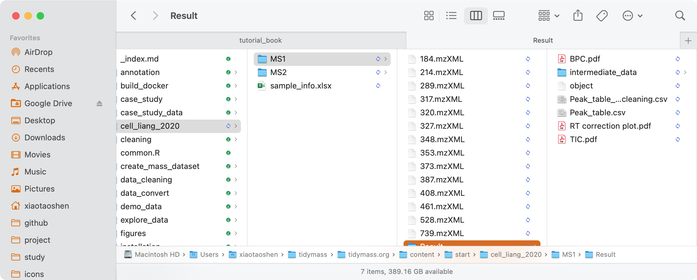
All the results will be placed in the folder named MS1/Result. More information about that can be found here.
-
BPC.pdf: BPC plot.
-
TIC.pdf: TIC plot.
-
RT correction plot.pdf: Retention time correction plot.
-
Peak_table.csv: Peak table.
-
Peak_table_for_cleaning.csv: Peak table which can be used for data cleaning.
-
object:
mass_datasetclass object which can be used for subsequent analysis using tidymass. -
intermediate_data: intermediate data.
You can just load the object, which is a mass_dataset class object.
load("cell_liang_2020/MS1/Result/object")
object
#> --------------------
#> massdataset version: 1.0.12
#> --------------------
#> 1.expression_data:[ 9164 x 14 data.frame]
#> 2.sample_info:[ 14 x 4 data.frame]
#> 14 samples:184 214 289 ... 528 739
#> 3.variable_info:[ 9164 x 3 data.frame]
#> 9164 variables:M71T823_POS M72T34_POS M72T822_POS ... M994T593_POS M995T593_POS
#> 4.sample_info_note:[ 4 x 2 data.frame]
#> 5.variable_info_note:[ 3 x 2 data.frame]
#> 6.ms2_data:[ 0 variables x 0 MS2 spectra]
#> --------------------
#> Processing information
#> 2 processings in total
#> create_mass_dataset ----------
#>       Package         Function.used                Time
#> 1 massdataset create_mass_dataset() 2022-08-08 07:44:32
#> process_data ----------
#>         Package Function.used                Time
#> 1 massprocesser  process_data 2022-08-08 07:44:28
dim(object)
#> variables   samples
#>      9164        14
We can get basic information from the object.
We have 9164 variables, 14 samples.
You can use the plot_adjusted_rt() function to get the interactive plot.
load("cell_liang_2020/MS1/Result/intermediate_data/xdata2")
####set the group_for_figure if you want to show specific groups.
####And set it as "all" if you want to show all samples.
plot <-
  plot_adjusted_rt(object = xdata2,
                   group_for_figure = "Subject",
                   interactive = TRUE)
plot
Explore data
After the raw data processing, peak tables will be generated.
load("cell_liang_2020/MS1/Result/object")
dim(object)
#> variables   samples
#>      9164        14
We neet to update the sample_info in object.
Read sample information.
sample_info <-
  readxl::read_xlsx("cell_liang_2020/sample_info.xlsx")
sample_info$sample_id <-
  as.character(sample_info$sample_id)
Add sample_info to object
object %>%
  extract_sample_info() %>%
  head()
#>   sample_id   group   class injection.order
#> 1       184 Subject Subject               1
#> 2       214 Subject Subject               2
#> 3       289 Subject Subject               3
#> 4       317 Subject Subject               4
#> 5       320 Subject Subject               5
#> 6       327 Subject Subject               6
object <-
  object %>%
  activate_mass_dataset(what = "sample_info") %>%
  left_join(sample_info,
            by = "sample_id")

object %>%
  extract_sample_info()
#>    sample_id   group   class injection.order subject_id trimester
#> 1        184 Subject Subject               1        aaf       >35
#> 2        214 Subject Subject               2        aaf       <10
#> 3        289 Subject Subject               3        ace       >35
#> 4        317 Subject Subject               4        acb       <10
#> 5        320 Subject Subject               5        abb       <10
#> 6        327 Subject Subject               6        aci       <10
#> 7        348 Subject Subject               7        abi       >35
#> 8        353 Subject Subject               8        abg       >35
#> 9        373 Subject Subject               9        aci       >35
#> 10       387 Subject Subject              10        abg       <10
#> 11       408 Subject Subject              11        abi       <10
#> 12       461 Subject Subject              12        acb       >35
#> 13       528 Subject Subject              13        abb       >35
#> 14       739 Subject Subject              14        ace       <10
object %>%
  activate_mass_dataset(what = "sample_info") %>%
  dplyr::count(class)
#>     class  n
#> 1 Subject 14

object %>%
  activate_mass_dataset(what = "sample_info") %>%
  dplyr::count(group)
#>     group  n
#> 1 Subject 14

object %>%
  activate_mass_dataset(what = "sample_info") %>%
  dplyr::count(trimester)
#>   trimester n
#> 1       <10 7
#> 2       >35 7
So for the data, we have 7 subjects and 14 samples. One subject has two samples.
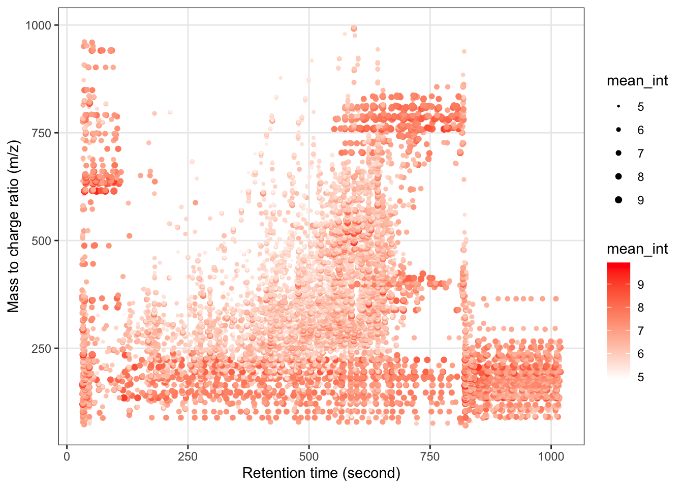
Next, we can get the peak distributation plot.
object %>%
  `+`(1) %>%
  log(10) %>%
  show_mz_rt_plot() +
  scale_size_continuous(range = c(0.01, 2))
We can explore the missing values in the data.
get_mv_number(object = object)
#> [1] 26696
sum(is.na(object))
#> [1] 26696
26,696 mvs in total.
Missing value number in each sample.
get_mv_number(object = object, by = "variable") %>%
  head()
#> M71T823_POS  M72T34_POS M72T822_POS  M73T36_POS M74T584_POS  M75T47_POS
#>           0           6           0           0           5           7
Missing value number in each variable.
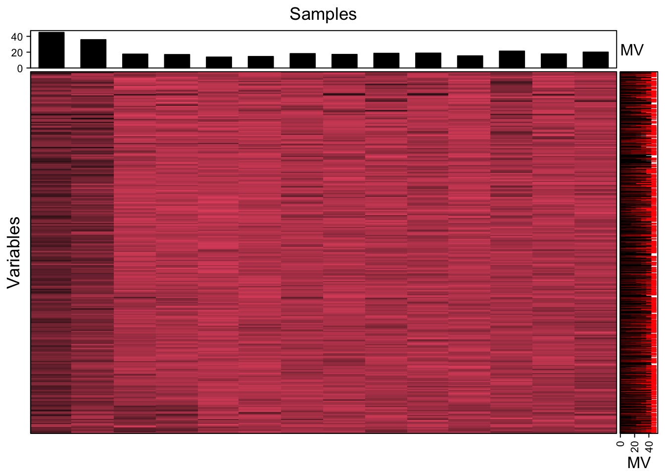
We can use the figure to show the missing value information.
show_missing_values(object = object,
                    show_column_names = FALSE, percentage = TRUE)
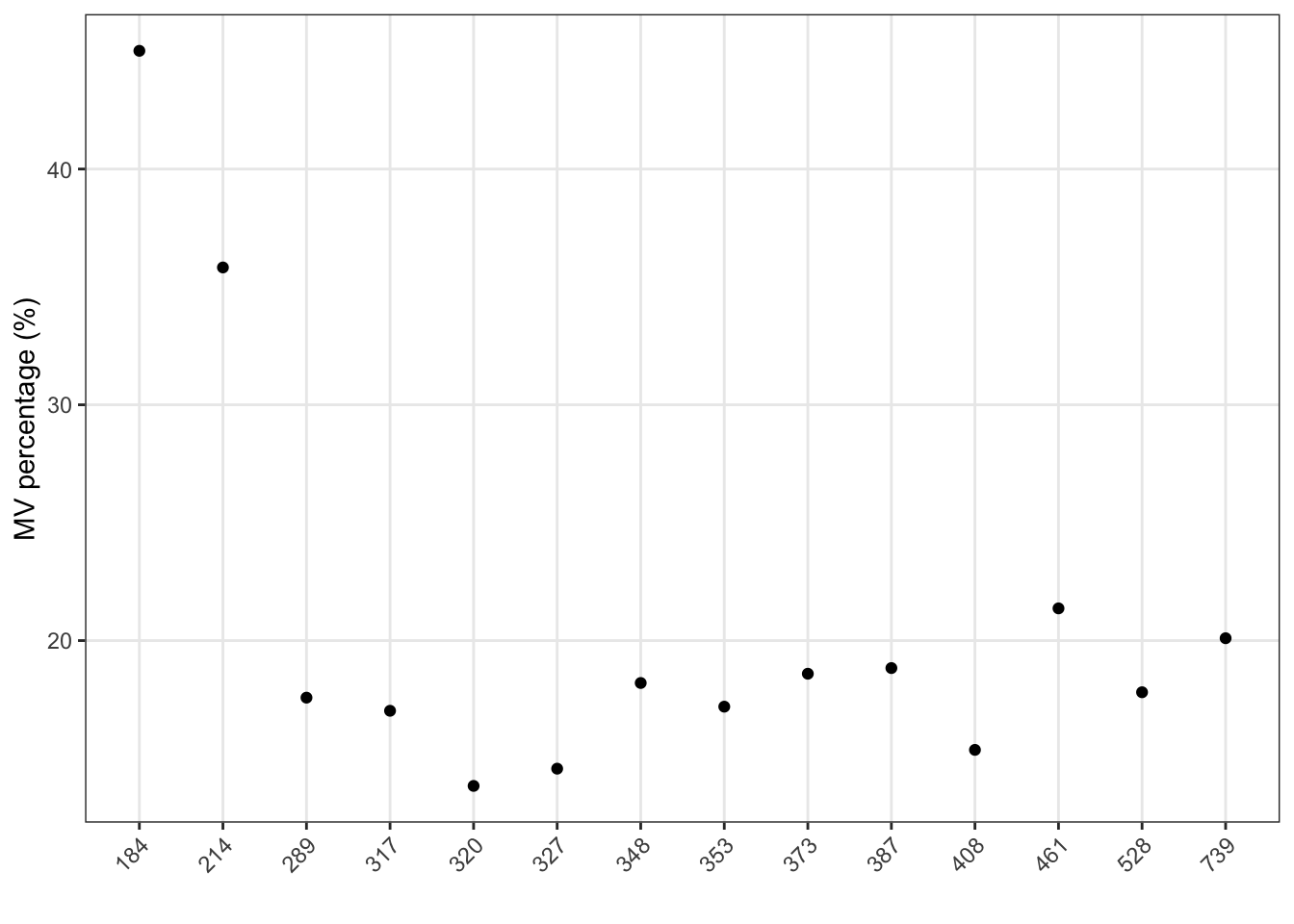
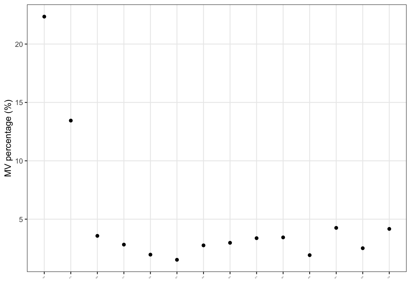
Show the mvs in samples
show_sample_missing_values(object = object, percentage = TRUE)
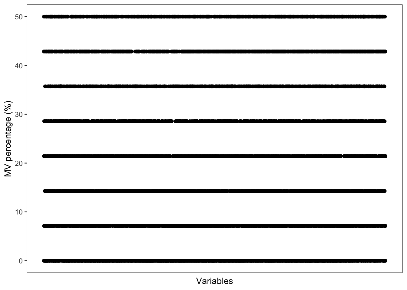
Show the mvs in variables
show_variable_missing_values(object = object,
                             percentage = TRUE,
                             show_x_text = FALSE,
                             show_x_ticks = FALSE) +
  scale_size_continuous(range = c(0.01, 1))
Data cleaning
Data quality assessment before data cleaning
Here, we can use the massqc package to assess the data quality.
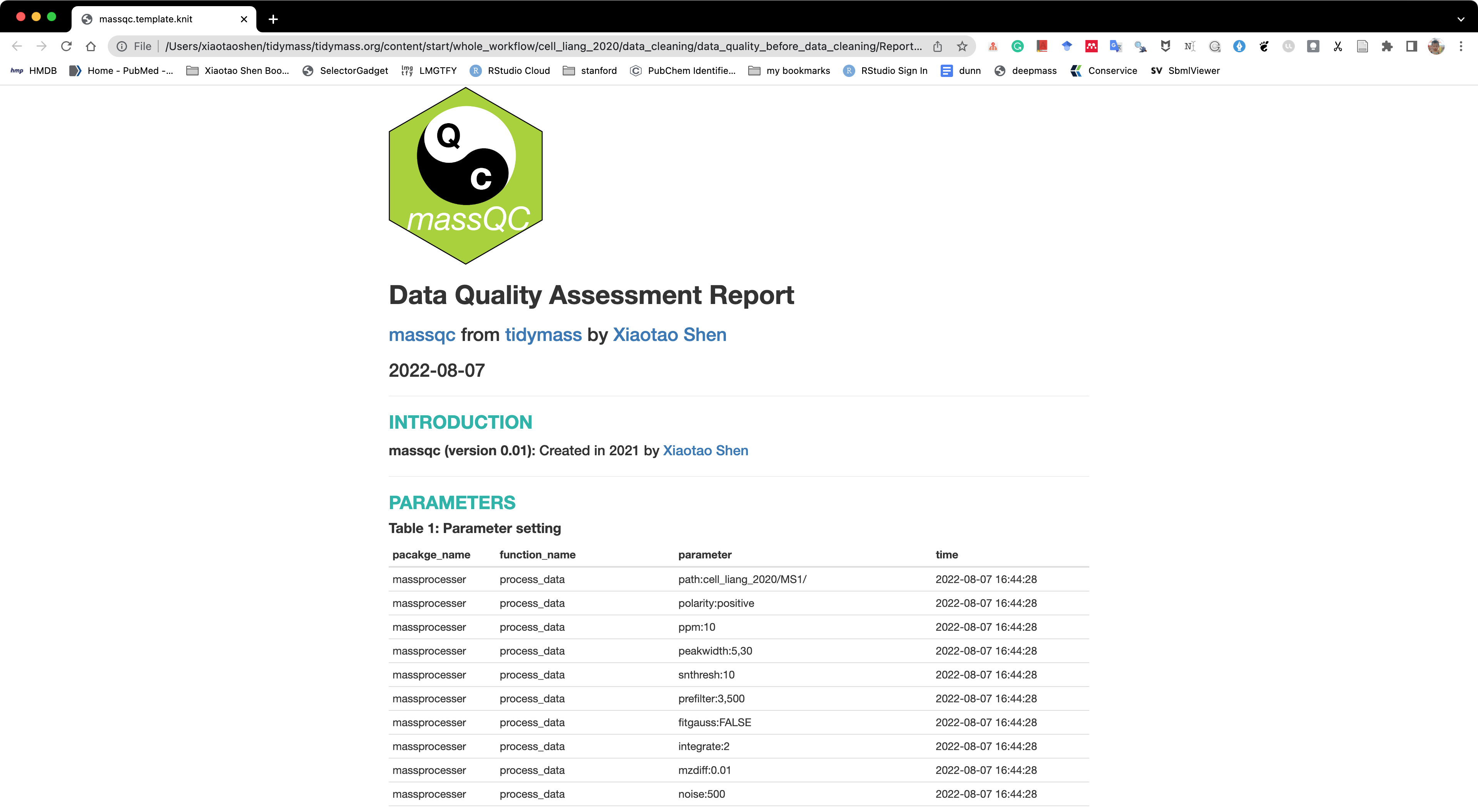
We can just use the massqc_report() function to get a html format quality assessment report.
massqc::massqc_report(object = object,
                      path = "cell_liang_2020/data_cleaning/data_quality_before_data_cleaning")
A html format report and pdf figures will be placed in the folder cell_liang_2020/data_cleaning/data_quality_before_data_cleaning/Report.
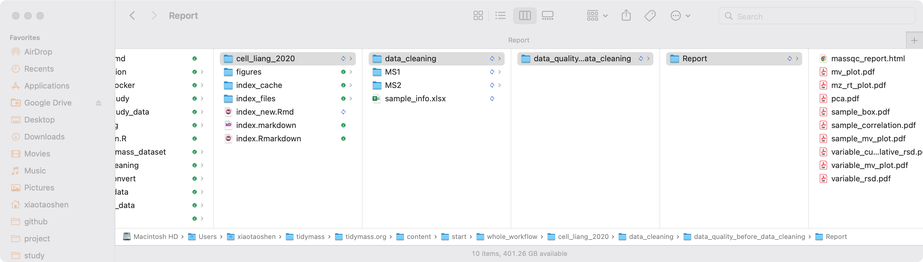
The html report is below:
Remove noisy metabolic features
Remove variables which have MVs in more than 20% samples.
show_variable_missing_values(object = object,
                             percentage = TRUE) +
  scale_size_continuous(range = c(0.01, 2))

object =
  object %>%
  mutate_variable_na_freq()

head(extract_variable_info(object))
#>   variable_id       mz        rt   na_freq
#> 1 M71T823_POS 70.98037 823.24475 0.0000000
#> 2  M72T34_POS 71.90757  33.84428 0.4285714
#> 3 M72T822_POS 71.98733 822.28662 0.0000000
#> 4  M73T36_POS 73.02834  36.06493 0.0000000
#> 5 M74T584_POS 73.70056 584.35419 0.3571429
#> 6  M75T47_POS 74.81906  46.72005 0.5000000
Remove variables.
object <-
  object %>%
  activate_mass_dataset(what = "variable_info") %>%
  filter(na_freq < 0.2)
dim(object)
#> variables   samples
#>      4537        14
Only 4,537 variables left.
Filter outlier samples
We can use the detect_outlier() to find the outlier samples.
More information about how to detect outlier samples can be found here.
massdataset::show_sample_missing_values(object = object,
                                        order_by = "injection.order",
                                        percentage = TRUE) +
  theme(axis.text.x = element_text(size = 2)) +
  scale_size_continuous(range = c(0.1, 2)) +
  ggsci::scale_color_aaas()
Detect outlier samples.
outlier_samples <-
  object %>%
  `+`(1) %>%
  log(2) %>%
  scale() %>%
  detect_outlier()

outlier_samples
#> --------------------
#> masscleaner
#> --------------------
#> 1 according_to_na : 0 outlier samples.
#> 2 according_to_pc_sd : 0 outlier samples.
#> 3 according_to_pc_mad : 1 outlier samples.
#> 184 .
#> 4 accordint_to_distance : 2 outlier samples.
#> 184,214 .
#> extract all outlier table using extract_outlier_table()
outlier_table <-
extract_outlier_table(outlier_samples)

outlier_table %>%
  head()
#>     according_to_na pc_sd pc_mad accordint_to_distance
#> 184           FALSE FALSE   TRUE                  TRUE
#> 214           FALSE FALSE  FALSE                  TRUE
#> 289           FALSE FALSE  FALSE                 FALSE
#> 317           FALSE FALSE  FALSE                 FALSE
#> 320           FALSE FALSE  FALSE                 FALSE
#> 327           FALSE FALSE  FALSE                 FALSE
No outlier samples according to NA.
Missing value imputation
get_mv_number(object)
#> [1] 3224
sum(is.na(object))
#> [1] 3224

object <-
  impute_mv(object = object, method = "knn")
#> Cluster size 4537 broken into 86 4451
#> Done cluster 86
#> Cluster size 4451 broken into 4168 283
#> Cluster size 4168 broken into 541 3627
#> Done cluster 541
#> Cluster size 3627 broken into 719 2908
#> Done cluster 719
#> Cluster size 2908 broken into 22 2886
#> Done cluster 22
#> Cluster size 2886 broken into 2097 789
#> Cluster size 2097 broken into 1365 732
#> Done cluster 1365
#> Done cluster 732
#> Done cluster 2097
#> Done cluster 789
#> Done cluster 2886
#> Done cluster 2908
#> Done cluster 3627
#> Done cluster 4168
#> Done cluster 283
#> Done cluster 4451

get_mv_number(object)
#> [1] 0
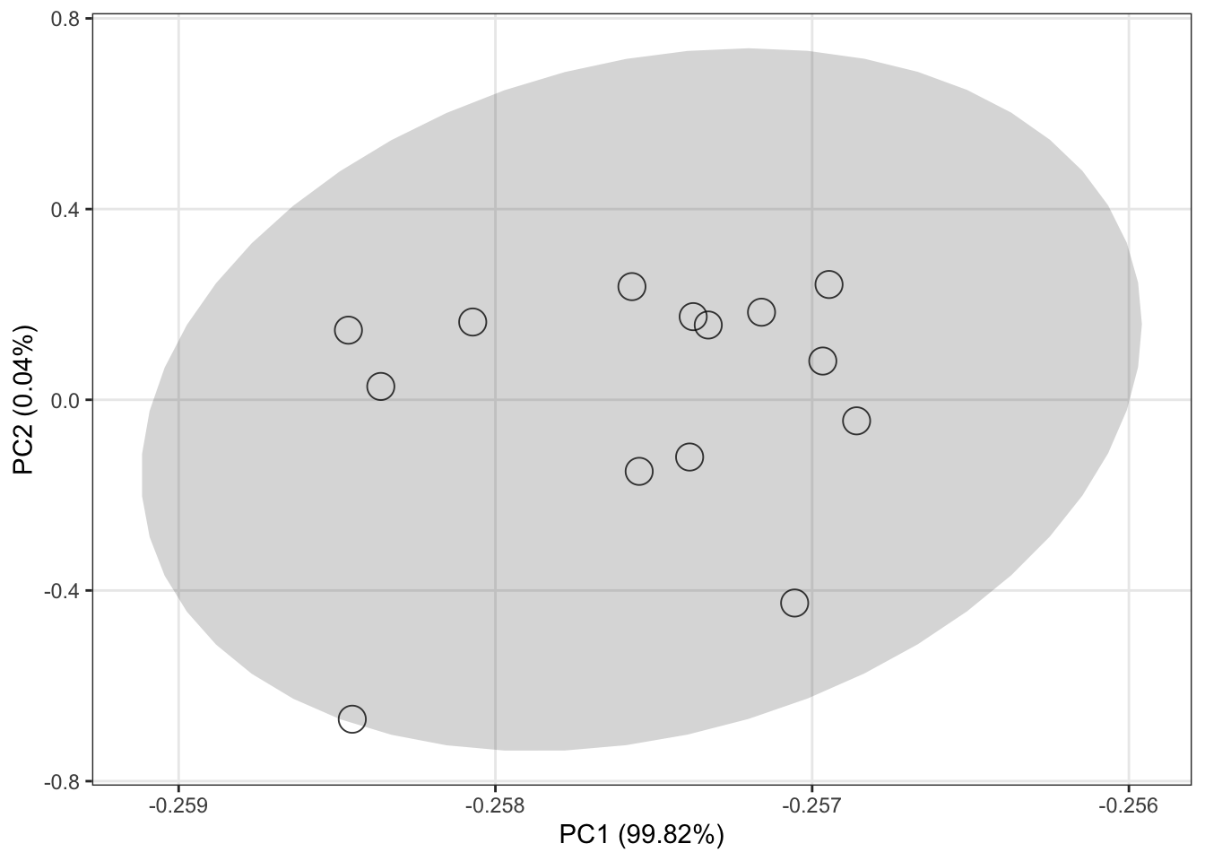
Data normalization and integration
object <-
  normalize_data(object, method = "median")
object %>%
  `+`(1) %>%
  log(2) %>%
  massqc::massqc_pca(line = FALSE)
Data quality assessment after data cleaning
Here, we can use the massqc package to assess the data quality.
We can just use the massqc_report() function to get a html format quality assessment report.
massqc::massqc_report(object = object,
                      path = "cell_liang_2020/data_cleaning/data_quality_after_data_cleaning")
Metabolite annotation
Add MS2 spectra to object
object <-
  mutate_ms2(
    object = object,
    column = "rp",
    polarity = "positive",
    ms1.ms2.match.mz.tol = 15,
    ms1.ms2.match.rt.tol = 30,
    path = "cell_liang_2020/MS2/"
  )
Metabolite annotation using metid
Metabolite annotation is based on the metid package.
Download database
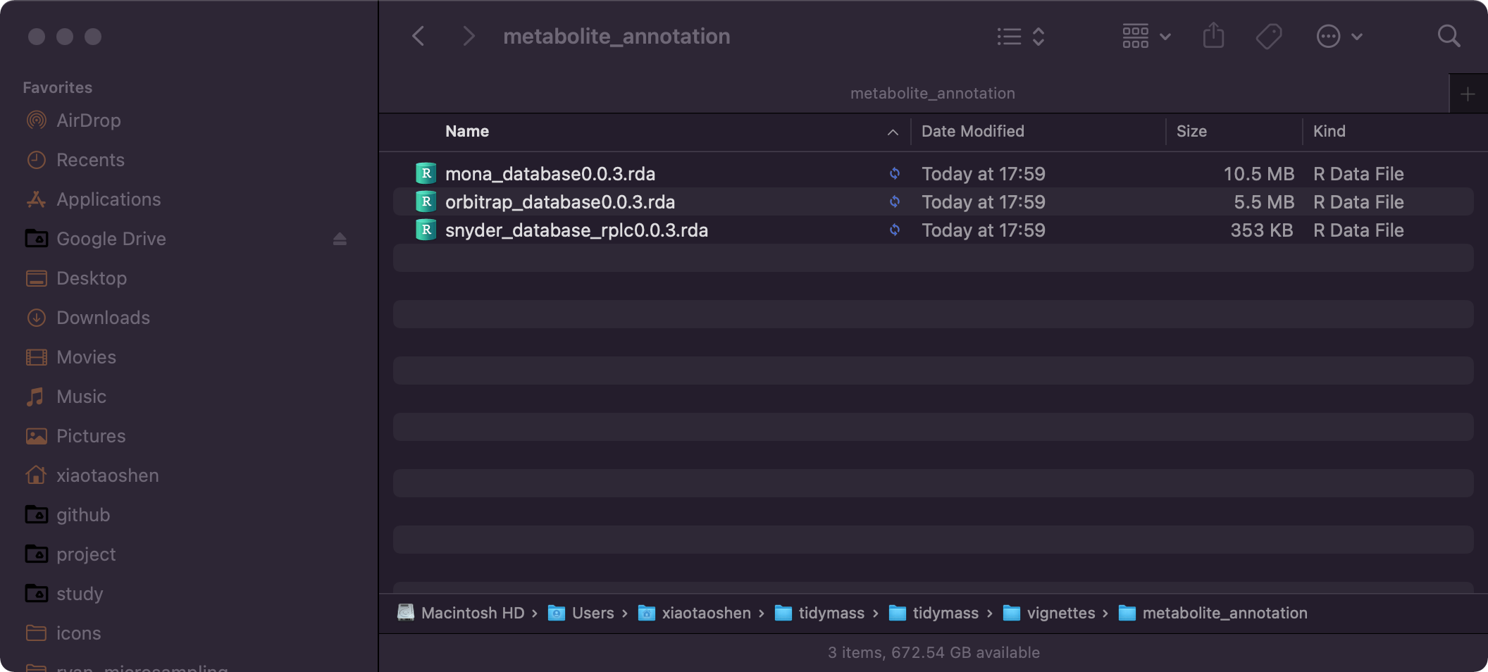
We need to download MS2 database from metid website.
Here we download the Michael Snyder RPLC databases, Orbitrap database and MoNA database. And place them in a new folder named as metabolite_annotation.
Annotate features using snyder_database_rplc0.0.3.
load("cell_liang_2020/metabolite_annotation/snyder_database_rplc0.0.3.rda")
object <-
  annotate_metabolites_mass_dataset(object = object,
                                    ms1.match.ppm = 15,
                                    rt.match.tol = 30,
                                    polarity = "positive",
                                    database = snyder_database_rplc0.0.3)
Annotate features using orbitrap_database0.0.3.
load("cell_liang_2020/metabolite_annotation/orbitrap_database0.0.3.rda")
object <-
  annotate_metabolites_mass_dataset(object = object,
                                    ms1.match.ppm = 15,
                                    polarity = "positive",
                                    database = orbitrap_database0.0.3)
Annotate features using mona_database0.0.3.
load("cell_liang_2020/metabolite_annotation/mona_database0.0.3.rda")
object <-
  annotate_metabolites_mass_dataset(object = object,
                                    ms1.match.ppm = 15,
                                    polarity = "positive",
                                    database = mona_database0.0.3)
Annotation result
head(extract_annotation_table(object = object))
#> data frame with 0 columns and 0 rows
variable_info <-
  extract_variable_info(object = object)
head(variable_info)
#>   variable_id       mz        rt    na_freq
#> 1 M71T823_POS 70.98037 823.24475 0.00000000
#> 2 M72T822_POS 71.98733 822.28662 0.00000000
#> 3  M73T36_POS 73.02834  36.06493 0.00000000
#> 4 M76T812_POS 76.10571 812.14087 0.14285714
#> 5  M77T33_POS 77.03845  32.64994 0.00000000
#> 6  M78T47_POS 77.96823  47.00970 0.07142857
table(variable_info$Level)
#> < table of extent 0 >
table(variable_info$Database)
#> < table of extent 0 >
ms2_plot_mass_dataset(object = object,
                      variable_id = "M123T56_POS",
                      database = snyder_database_rplc0.0.3)
Statistical analysis
Remove the features without annotations
object <-
  object %>%
  activate_mass_dataset(what = "annotation_table") %>%
  filter(!is.na(Level)) %>%
  filter(Level == 1 | Level == 2)
object
#> --------------------
#> massdataset version: 1.0.12
#> --------------------
#> 1.expression_data:[ 4537 x 14 data.frame]
#> 2.sample_info:[ 14 x 6 data.frame]
#> 14 samples:184 214 289 ... 528 739
#> 3.variable_info:[ 4537 x 4 data.frame]
#> 4537 variables:M71T823_POS M72T822_POS M73T36_POS ... M993T593_POS M994T593_POS
#> 4.sample_info_note:[ 6 x 2 data.frame]
#> 5.variable_info_note:[ 4 x 2 data.frame]
#> 6.ms2_data:[ 0 variables x 0 MS2 spectra]
#> --------------------
#> Processing information
#> 6 processings in total
#> Latest 3 processings show
#> filter ----------
#>       Package Function.used                Time
#> 1 massdataset      filter() 2024-09-25 17:21:18
#> impute_mv ----------
#>       Package Function.used                Time
#> 1 masscleaner   impute_mv() 2024-09-25 17:21:18
#> normalize_data ----------
#>       Package    Function.used                Time
#> 1 masscleaner normalize_data() 2024-09-25 17:21:18
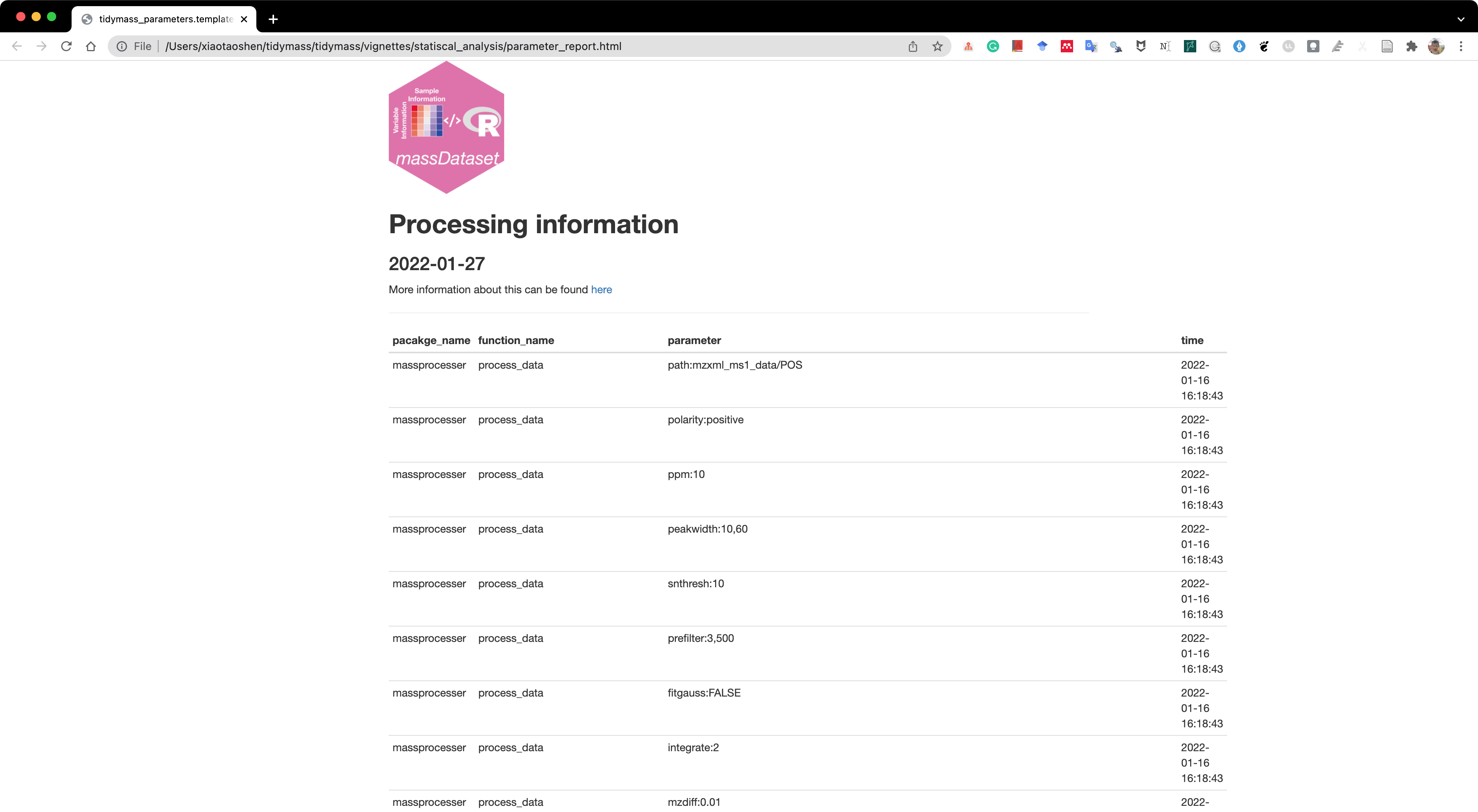
Trace processing information of object
Then we can use the report_parameters() function to trace processing information of object.
All the analysis results will be placed in a folder named as statistical_analysis.
dir.create(path = "cell_liang_2020/statistical_analysis", showWarnings = FALSE)
report_parameters(object = object, path = "cell_liang_2020/statistical_analysis/")
A html format file named as parameter_report.html will be generated.
Remove redundant metabolites
Remove the redundant annotated metabolites bases on Level and score.
object <-
  object %>%
  activate_mass_dataset(what = "annotation_table") %>%
  group_by(Compound.name) %>%
  filter(Level == min(Level)) %>%
  filter(SS == max(SS)) %>%
  slice_head(n = 1)
Differential expression metabolites
Calculate the fold changes.
object <-
  object %>%
  activate_mass_dataset(what = "sample_info") %>%
  dplyr::arrange(subject_id, trimester)

control_sample_id <-
  object %>%
  activate_mass_dataset(what = "sample_info") %>%
  filter(trimester == "<10") %>%
  pull(sample_id)

case_sample_id <-
  object %>%
  activate_mass_dataset(what = "sample_info") %>%
  filter(trimester == ">35") %>%
  pull(sample_id)
object <-
  mutate_fc(object = object,
            control_sample_id = control_sample_id,
            case_sample_id = case_sample_id,
            mean_median = "mean")
Calculate p values.
object <-
  mutate_p_value(
    object = object,
    control_sample_id = control_sample_id,
    case_sample_id = case_sample_id,
    method = "wilcox.test",
    p_adjust_methods = "BH",
    paired = TRUE
  )
Volcano plot.
volcano_plot(object = object,
             add_text = TRUE,
             text_from = "Compound.name",
             point_size_scale = "p_value") +
  scale_size_continuous(range = c(0.5, 5))
Output result
Output the differential expression metabolites.
differential_metabolites <-
  extract_variable_info(object = object) %>%
  filter(fc > 2 | fc < 0.5) %>%
  filter(p_value_adjust < 0.05)

readr::write_csv(differential_metabolites,
                 file = "cell_liang_2020/statistical_analysis/differential_metabolites.csv")
Pathway enrichment analysis
All the results will be placed in a folder named as pathway_enrichment.
dir.create(path = "cell_liang_2020/pathway_enrichment", showWarnings = FALSE)
diff_metabolites <-
  object %>%
  activate_mass_dataset(what = "variable_info") %>%
  filter(p_value_adjust < 0.05) %>%
  extract_variable_info()
head(diff_metabolites)
Load KEGG human pathway database
data("kegg_hsa_pathway", package = "metpath")
kegg_hsa_pathway
get_pathway_class(kegg_hsa_pathway)
Remove the disease pathways:
#get the class of pathways
pathway_class <-
  metpath::pathway_class(kegg_hsa_pathway)
head(pathway_class)
remain_idx <-
  pathway_class %>%
  unlist() %>%
  stringr::str_detect("Disease") %>%
  `!`() %>%
  which()

remain_idx
pathway_database <-
  kegg_hsa_pathway[remain_idx]
pathway_database
Pathway enrichment
kegg_id <-
  diff_metabolites$KEGG.ID
kegg_id <-
  kegg_id[!is.na(kegg_id)]
kegg_id
result <-
enrich_kegg(query_id = kegg_id,
            query_type = "compound",
            id_type = "KEGG",
            pathway_database = pathway_database,
            p_cutoff = 0.05,
            p_adjust_method = "BH",
            threads = 3)
Check the result:
result
Plot to show pathway enrichment result
enrich_bar_plot(object = result,
                x_axis = "p_value",
                cutoff = 0.05)
enrich_scatter_plot(object = result, y_axis = "p_value", y_axis_cutoff = 0.05)
enrich_network(
  object = result,
  point_size = "p_value",
  p_cutoff = 0.05,
  only_significant_pathway = TRUE
)
Session information
sessionInfo()
#> R version 4.4.1 (2024-06-14)
#> Platform: aarch64-apple-darwin20
#> Running under: macOS 15.0
#>
#> Matrix products: default
#> BLAS:   /Library/Frameworks/R.framework/Versions/4.4-arm64/Resources/lib/libRblas.0.dylib
#> LAPACK: /Library/Frameworks/R.framework/Versions/4.4-arm64/Resources/lib/libRlapack.dylib;  LAPACK version 3.12.0
#>
#> locale:
#> [1] en_US.UTF-8/en_US.UTF-8/en_US.UTF-8/C/en_US.UTF-8/en_US.UTF-8
#>
#> time zone: Asia/Singapore
#> tzcode source: internal
#>
#> attached base packages:
#> [1] grid      stats4    stats     graphics  grDevices utils     datasets
#> [8] methods   base
#>
#> other attached packages:
#>  [1] lubridate_1.9.3       forcats_1.0.0         stringr_1.5.1
#>  [4] purrr_1.0.2           readr_2.1.5           tibble_3.2.1
#>  [7] tidyverse_2.0.0       metid_1.2.33          metpath_1.0.8
#> [10] ComplexHeatmap_2.20.0 mixOmics_6.28.0       lattice_0.22-6
#> [13] MASS_7.3-61           massstat_1.0.6        tidyr_1.3.1
#> [16] ggfortify_0.4.17      massqc_1.0.7          masscleaner_1.0.12
#> [19] MSnbase_2.30.1        ProtGenerics_1.36.0   S4Vectors_0.42.1
#> [22] Biobase_2.64.0        BiocGenerics_0.50.0   mzR_2.38.0
#> [25] Rcpp_1.0.13           xcms_4.2.3            BiocParallel_1.38.0
#> [28] massprocesser_1.0.10  ggplot2_3.5.1         dplyr_1.1.4
#> [31] magrittr_2.0.3        masstools_1.0.13      massdataset_1.0.34
#> [34] tidymass_1.0.9
#>
#> loaded via a namespace (and not attached):
#>   [1] fs_1.6.4                    matrixStats_1.3.0
#>   [3] bitops_1.0-8                fit.models_0.64
#>   [5] httr_1.4.7                  RColorBrewer_1.1-3
#>   [7] doParallel_1.0.17           ggsci_3.2.0
#>   [9] tools_4.4.1                 doRNG_1.8.6
#>  [11] backports_1.5.0             utf8_1.2.4
#>  [13] R6_2.5.1                    lazyeval_0.2.2
#>  [15] GetoptLong_1.0.5            withr_3.0.1
#>  [17] prettyunits_1.2.0           gridExtra_2.3
#>  [19] preprocessCore_1.66.0       cli_3.6.3
#>  [21] Cairo_1.6-2                 fastDummies_1.7.4
#>  [23] labeling_0.4.3              sass_0.4.9
#>  [25] mvtnorm_1.3-1               robustbase_0.99-4
#>  [27] randomForest_4.7-1.1        proxy_0.4-27
#>  [29] pbapply_1.7-2               foreign_0.8-87
#>  [31] rrcov_1.7-6                 MetaboCoreUtils_1.12.0
#>  [33] parallelly_1.38.0           itertools_0.1-3
#>  [35] limma_3.60.4                readxl_1.4.3
#>  [37] rstudioapi_0.16.0           impute_1.78.0
#>  [39] generics_0.1.3              shape_1.4.6.1
#>  [41] zip_2.3.1                   Matrix_1.7-0
#>  [43] MALDIquant_1.22.3           fansi_1.0.6
#>  [45] abind_1.4-5                 lifecycle_1.0.4
#>  [47] yaml_2.3.10                 SummarizedExperiment_1.34.0
#>  [49] SparseArray_1.4.8           crayon_1.5.3
#>  [51] PSMatch_1.8.0               KEGGREST_1.44.1
#>  [53] magick_2.8.4                pillar_1.9.0
#>  [55] knitr_1.48                  GenomicRanges_1.56.1
#>  [57] rjson_0.2.22                corpcor_1.6.10
#>  [59] codetools_0.2-20            glue_1.7.0
#>  [61] pcaMethods_1.96.0           data.table_1.16.0
#>  [63] remotes_2.5.0               MultiAssayExperiment_1.30.3
#>  [65] vctrs_0.6.5                 png_0.1-8
#>  [67] cellranger_1.1.0            gtable_0.3.5
#>  [69] cachem_1.1.0                xfun_0.47
#>  [71] openxlsx_4.2.7              S4Arrays_1.4.1
#>  [73] tidygraph_1.3.1             pcaPP_2.0-5
#>  [75] ncdf4_1.23                  iterators_1.0.14
#>  [77] statmod_1.5.0               robust_0.7-5
#>  [79] progress_1.2.3              GenomeInfoDb_1.40.1
#>  [81] rprojroot_2.0.4             bslib_0.8.0
#>  [83] affyio_1.74.0               rpart_4.1.23
#>  [85] colorspace_2.1-1            DBI_1.2.3
#>  [87] Hmisc_5.1-3                 nnet_7.3-19
#>  [89] tidyselect_1.2.1            compiler_4.4.1
#>  [91] MassSpecWavelet_1.70.0      htmlTable_2.4.3
#>  [93] DelayedArray_0.30.1         plotly_4.10.4
#>  [95] bookdown_0.40               checkmate_2.3.2
#>  [97] scales_1.3.0                DEoptimR_1.1-3
#>  [99] affy_1.82.0                 digest_0.6.37
#> [101] rmarkdown_2.28              XVector_0.44.0
#> [103] htmltools_0.5.8.1           pkgconfig_2.0.3
#> [105] base64enc_0.1-3             MatrixGenerics_1.16.0
#> [107] highr_0.11                  fastmap_1.2.0
#> [109] rlang_1.1.4                 GlobalOptions_0.1.2
#> [111] htmlwidgets_1.6.4           UCSC.utils_1.0.0
#> [113] farver_2.1.2                jquerylib_0.1.4
#> [115] jsonlite_1.8.8              MsExperiment_1.6.0
#> [117] mzID_1.42.0                 RCurl_1.98-1.16
#> [119] Formula_1.2-5               GenomeInfoDbData_1.2.12
#> [121] patchwork_1.2.0             munsell_0.5.1
#> [123] viridis_0.6.5               MsCoreUtils_1.16.1
#> [125] vsn_3.72.0                  furrr_0.3.1
#> [127] stringi_1.8.4               ggraph_2.2.1
#> [129] zlibbioc_1.50.0             plyr_1.8.9
#> [131] parallel_4.4.1              listenv_0.9.1
#> [133] ggrepel_0.9.5               Biostrings_2.72.1
#> [135] MsFeatures_1.12.0           graphlayouts_1.1.1
#> [137] hms_1.1.3                   Spectra_1.14.1
#> [139] circlize_0.4.16             igraph_2.0.3
#> [141] QFeatures_1.14.2            rngtools_1.5.2
#> [143] reshape2_1.4.4              XML_3.99-0.17
#> [145] evaluate_0.24.0             blogdown_1.19
#> [147] BiocManager_1.30.25         tzdb_0.4.0
#> [149] foreach_1.5.2               missForest_1.5
#> [151] tweenr_2.0.3                polyclip_1.10-7
#> [153] future_1.34.0               clue_0.3-65
#> [155] ggforce_0.4.2               AnnotationFilter_1.28.0
#> [157] e1071_1.7-14                RSpectra_0.16-2
#> [159] ggcorrplot_0.1.4.1          viridisLite_0.4.2
#> [161] class_7.3-22                rARPACK_0.11-0
#> [163] memoise_2.0.1               ellipse_0.5.0
#> [165] IRanges_2.38.1              cluster_2.1.6
#> [167] timechange_0.3.0            globals_0.16.3
#> [169] here_1.0.1