Data normalization and integration
Xiaotao Shen PhD (https://www.shenxt.info/)
true
Created on 2020-04-01 and updated on 2021-04-07
Source:vignettes/data_normalization_integration.Rmd
data_normalization_integration.RmdWe can use metflow2 for data normalization and data integration.
First, we need to prepare samples for metflow2.
Data preparation
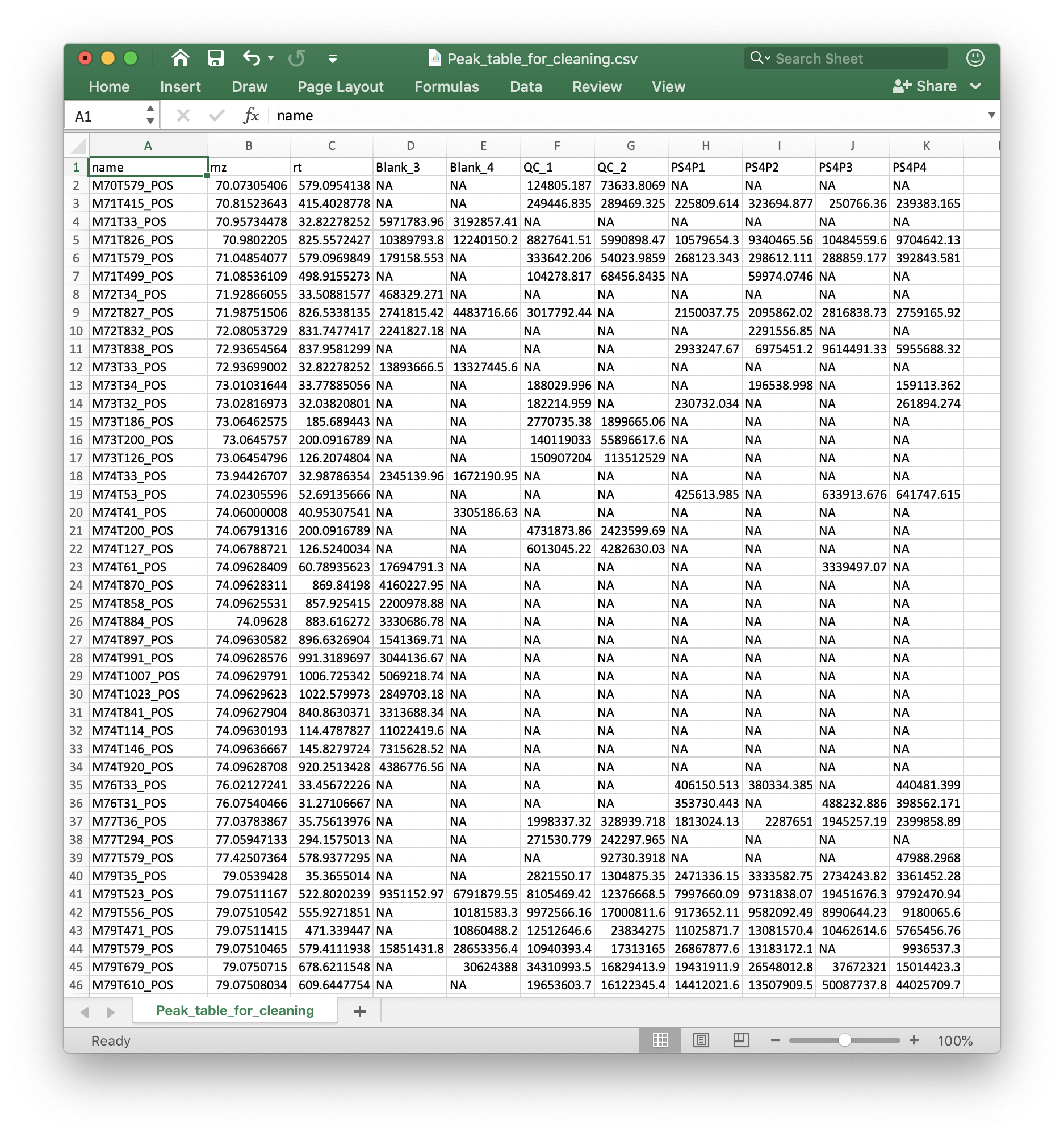
Peak table
The peak table (csv format) can be from any software. We recomment that you use the Peak_table_for_cleaning.csv from processData() function from metflow2.
If you use other software, please make sure that the top 3 columns are name (peak name), mz and rt (rentention time, second). And the left column are sample intensity.
Read data
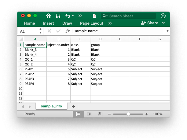
Then place the peak table and sample information in a folder. We use the demo data from demoData package.
Load demo data
##create a folder named as example
path <- file.path(".", "example")
dir.create(path = path, showWarnings = FALSE)
##get demo data
demo_data <- system.file("metflow2", package = "demoData")

file.copy(from = file.path(demo_data, dir(demo_data)),
          to = path, overwrite = TRUE, recursive = TRUE)
#> [1] TRUE TRUE TRUE TRUE TRUE
Here, we have two peak tables, batch1.data.csv and batch2.data.csv, and sample_info.csv are in your ./example folder.
Create metflowClass object
object <-
  create_metflow_object(
    ms1.data = c("batch1.data.csv", "batch2.data.csv"),
    sample.information = "sample_info.csv",
    path = path
  )
#> `creatMetflowObject()` is deprecated, please use `create_metflow_object()`Reading data...
#> --------------------------------------------------------------
#> --------------------------------------------------------------
#> --------------------------------------------------------------
#> Summary:
#>             Check result OK Warning Error
#> batch1             Valid  3       0     0
#> batch2             Valid  3       0     0
#> sample.info        Valid  9       0     0
#>
#>
#> data:
#> Batch 1 is valid.
#> Batch 2 is valid.
#>
#> sample.info:
#> sample.info is valid.
object is a metflowClass object, so you can print it in the console.
Align different batches
Because there are two batch peak tables, so first we must align them.
object <- align_batch(
  object = object,
  combine.mz.tol = 15,
  combine.rt.tol = 30,
  use.int.tol = FALSE
)
#> Rough aligning...
#> Accurate aligning...
Missing value processing
Remove noisy peaks and outlier samples
object2 <- filter_peaks(
  object = object,
  min.fraction = 0.5,
  type = "any",
  min.subject.blank.ratio = 2,
  according.to = "class",
  which.group = "QC"
)
#> QC are in the class .
#> --------------------
#> Removing peaks according to NA in samples...
#> 353 out of 354 peaks are remained.
#> --------------------
#> Removing peaks according to blank samples...
#> No Blanks in your data.
#> --------------------
#> Removing peaks according to QC dilution samples...
#> All done.
Remove outlier samples
Nest, we should remove some samples which have a lot of missing values.
object2 <- filter_samples(object = object2,
                          min.fraction.peak = 0.9)
#> Samples with MV ratio larger than 0.1 :
#>  EC567; EC5A1395; EC4604; EC7542; EC7528; EC6345; EC34A1771; ECA1469; EC24A1581; ECA558; EC6513; EC4385; EC6305; EC6893; EC8289; ECFA123; EC6894; EC3768; EC4286; EC8457; EC4054; EC4193; EC4483; EC7371; EC4171; EC6358; EC4052; EC6731; EC4771; ECA1356; EC6109; EC4086; EC4600; EC4272; EC7527; EC4338; EC47A2049; EC4602; EC6559; EC6304; EC4201; EC4135; EC4105; EC4532; EC4235; EC3703; EC8367; EC3688; EC7603; EC6562; EC6402; EC32A1737; EC7244; EC6634; EC8065; EC3938; EC3687; EC4224; EC4348; EC7154; EC4619; EC25A1596; EC7549; EC4220; EC6103; EC4268; ECA1318; EC3944; EC3677; EC25A1594; EC6202; EC4270; EC3826; EC7599; EC6408; EC6A1200; ECFB147; EC4349; EC7415; ECFD103; EC3972; EC6120; EC6561; EC7522; EC6594; EC53A2215; EC47A2046; EC6557; EC6517; EC4365; EC4455; EC17A1458; EC4641; EC6364; EC7460; EC6891; ECA1467; EC4121; EC6A1215; EC6349; EC7447; EC4177; EC26A1605; EC7586; EC6591; EC30A1671; EC4370; EC4654; EC4374; EC4565; EC563; EC3751; ECFB60; EC7631; EC4638; EC8365; EC4149; EC4536; EC4293; ECFB123_1; EC7403; EC4302; EC6291; EC6461; EC6742; EC7597; EC6748; EC6101; EC4106; EC4265; EC4136; EC4206; EC7372; EC6208; EC6752; EC4482; EC7590; EC4781; EC7234; EC7458; EC7438; EC6200_1; EC6459; EC6902; EC6326; EC4173; ECFA125; EC8363; ECFC120; EC4179; EC4493; EC7446; EC6290; EC4382; EC6112; EC7577; EC4160; EC7160; EC3670; EC8056_1; ECFB129; EC7536; ECFC18; EC0552; ECA111; EC7274; EC618; EC619; ECA168; ECA225; EC6840; EC6857; EC6926; ECA004; EC0628_1; ECA162; EC7135; ECA424; EC625; ECA222; EC7514; EC8551; ECA220; EC6953; ECA507; ECA201; ECA102; ECA1088; EC0909; ECA504; EC7064; EC656; EC7570; EC0753; ECA137; ECA1161; EC7490; ECA301; EC6849; ECA100; EC6864; EC6988; EC7031; ECA299; EC7482; EC636; EC738; EC0890; EC7470; EC686; EC0356; EC7025; ECA195; EC687; ECA188; EC628; EC7143; EC611; EC4A1168; EC6938; EC7084; EC7139; EC620; EC6812; ECA097; EC595; EC0848; EC7511; ECA041; EC7327; EC6843; EC655; ECA297; ECA176; EC632; ECA328; ECA287; EC237; ECA125; EC7515; ECA038; ECA120; ECA217; EC7101; EC7492; ECA239; EC7392; EC7276; ECA214; EC7009; EC189; ECA408; ECA212; EC0114; ECA126; ECA121; ECA286; EC7063; EC7384; EC627_1; EC6934; EC6907; ECFC145; EC7454; ECA107; EC6758; EC7355; EC6913; ECA210; EC7285; ECA573; ECA327; EC7502; ECA098; ECA197; ECA169; ECA288; EC616; ECA642; ECA537; EC7286; ECA290; ECA193; EC0858; ECA405; ECA407; ECA167; EC6915; EC7183; ECA108; EC0466; ECA425; ECA1070; EC302; ECA106; EC7507; EC735; EC7070; EC623; EC7184; EC577; EC0830; EC0576; ECA508; EC612; EC7393; EC6993; EC633; ECA110; EC0864; ECA574; EC6945; ECA418; EC653; EC7114; EC1A1079; EC711_1; EC646; EC0681; ECA186; ECA143; EC733; ECA103; ECA022; EC7061; ECA1142; ECA216; ECA024; ECA415
#> All done!
Missing value imputation
object2 <- impute_mv(object = object2,
                    method = "knn")
object2
#> --------------------
#> metflow2 version: 0.1.0
#> --------------------
#> MS1 data
#> There are 1 peak tables in your MS1 data.
#>        Peak.number Column.number
#> Batch1         353           108
#> --------------------
#> There are 105 samples in your MS1 data.
#>     Class Number
#> 1      QC     50
#> 2 Subject     55
#> --------------------
#>   Group Number
#> 1     0      5
#> 2     1     50
#> 3    QC     50
#> --------------------
#> Processing
#> alignBatch ----------
#>        Parameter Value
#> 1 combine.mz.tol    15
#> 2 combine.rt.tol    30
#> filterPeaks ----------
#>      Parameter Value
#> 1 min.fraction   0.5
#> 2  which.group    QC
#> filterSample ----------
#>           Parameter Value
#> 1 min.fraction.peak   0.9
#> imputeMV ----------
#>     Parameter     Value
#> 1      method       knn
#> 2           k        10
#> 3      rowmax       0.5
#> 4      colmax       0.8
#> 5        maxp      1500
#> 6    rng.seed 362436069
#> 7     maxiter        10
#> 8       ntree       100
#> 9  decreasing     FALSE
#> 10       nPcs         2
#> 11   maxSteps       100
#> 12  threshold     1e-04
#> combine.mz.tol

#> combine.rt.tol
#> min.fraction

#> which.group
#> 0.5

#> QC
#> min.fraction.peak
#> method

#> k

#> rowmax

#> colmax

#> maxp

#> rng.seed

#> maxiter

#> ntree

#> decreasing

#> nPcs

#> maxSteps

#> threshold
#> knn

#> 10

#> 0.5

#> 0.8

#> 1500

#> 362436069

#> 10

#> 100

#> FALSE

#> 2

#> 100

#> 1e-04
Data normalization
Now we can normalize data using different methods.
object3 <- normalize_data(object = object2, method = "mean")object3 <- normalize_data(object = object2, method = "svr", threads = 1)
#> Batch 1 ...
#>
|
| | 0%
|
|======================================================================| 100%
#>
#> SVR normalization is done
#>
#> Batch 2 ...
#>
|
| | 0%
|
|======================================================================| 100%
#>
#> SVR normalization is done
# object3 <- normalize_data(object = object2, method = "pqn")After data normaliztion, you can use the get_peak_int_distribution() function to see each peak intensity distributation plot.
get_peak_int_distribution(object = object3, peak_name = "M114T670", interactive = TRUE)
get_peak_int_distribution(object = object2, peak_name = "M114T670", interactive = TRUE)Data integration
Then we can use the integrate_data() function to do data integration.
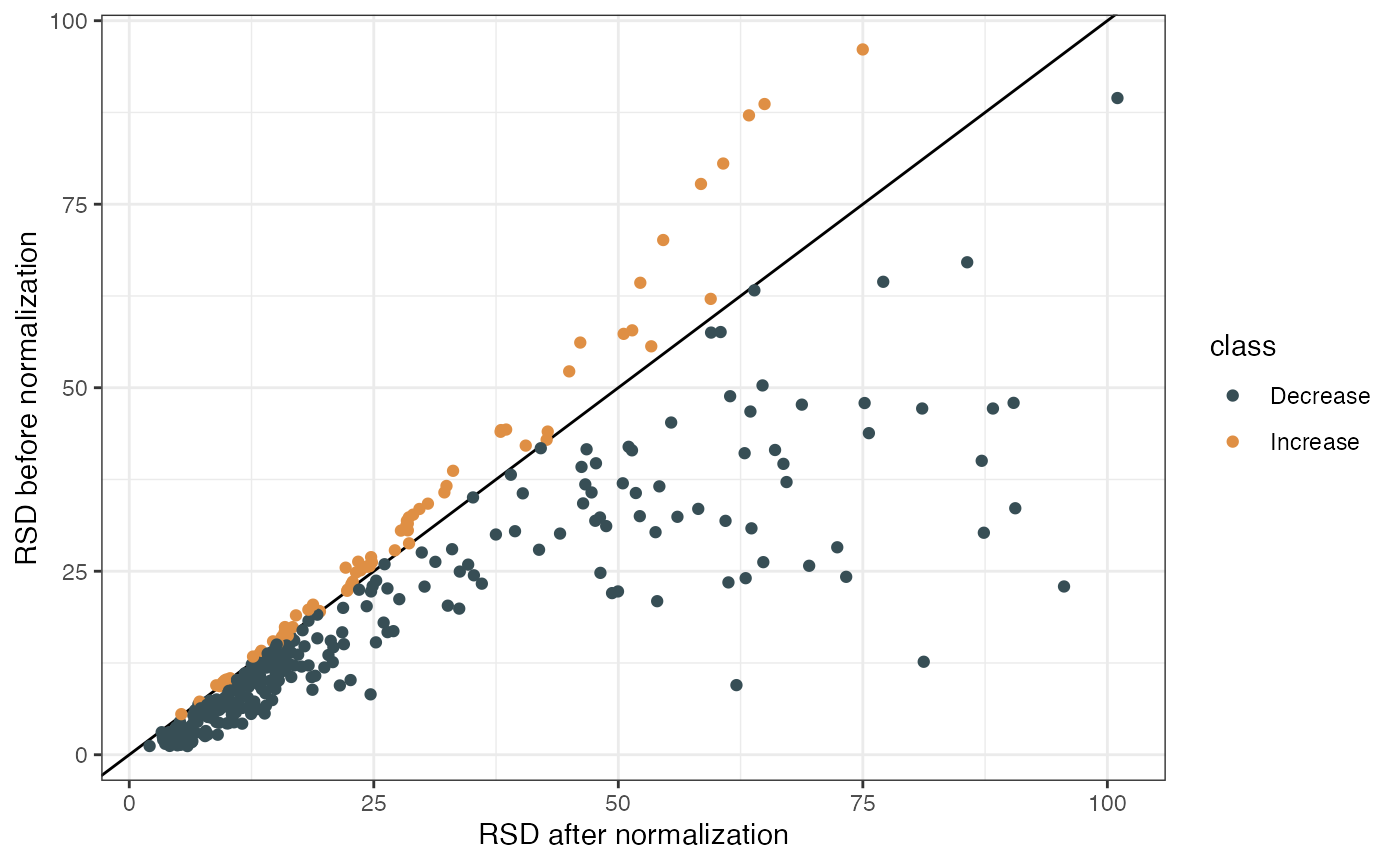
object4 <- integrate_data(object = object3, method = "qc.mean")We can also get the RSDs of all the peaks before and after data normalization and data integration.
rsd2 <- calculate_rsd(object = object2, slot = "QC")
rsd4 <- calculate_rsd(object = object4, slot = "QC")
Then we can draw the comprison plot:
library(ggplot2)
dplyr::left_join(rsd2, rsd4, by = c("index", "name")) %>%
  dplyr::mutate(class = dplyr::case_when(rsd.y < rsd.x ~ "Decrease",
                                         rsd.y > rsd.x ~ "Increase",
                                         rsd.y == rsd.y ~ "Equal")) %>%
  ggplot(aes(rsd.x, rsd.y, colour = class)) +
  ggsci::scale_color_jama() +
  geom_abline(slope = 1, intercept = 0) +
  geom_point() +
  labs(x = "RSD after normalization", y = "RSD before normalization") +
  theme_bw()