10 Subnetwork Extraction
This chapter focuses on how to use Step 3: PCSF Subnetwork in FeatureMAP Shiny. The detailed method, parameter definitions, and result structure have already been introduced in R package-Subnetwork Extraction, so here we focus on the Shiny workflow itself.
Prerequisites: Make sure Feature Annotation has finished successfully before starting this step.
10.1 Enter the PCSF Subnetwork Page
After finishing Feature Annotation, click Next Step, or open Analysis → 3 PCSF Subnetwork in the navigation bar.
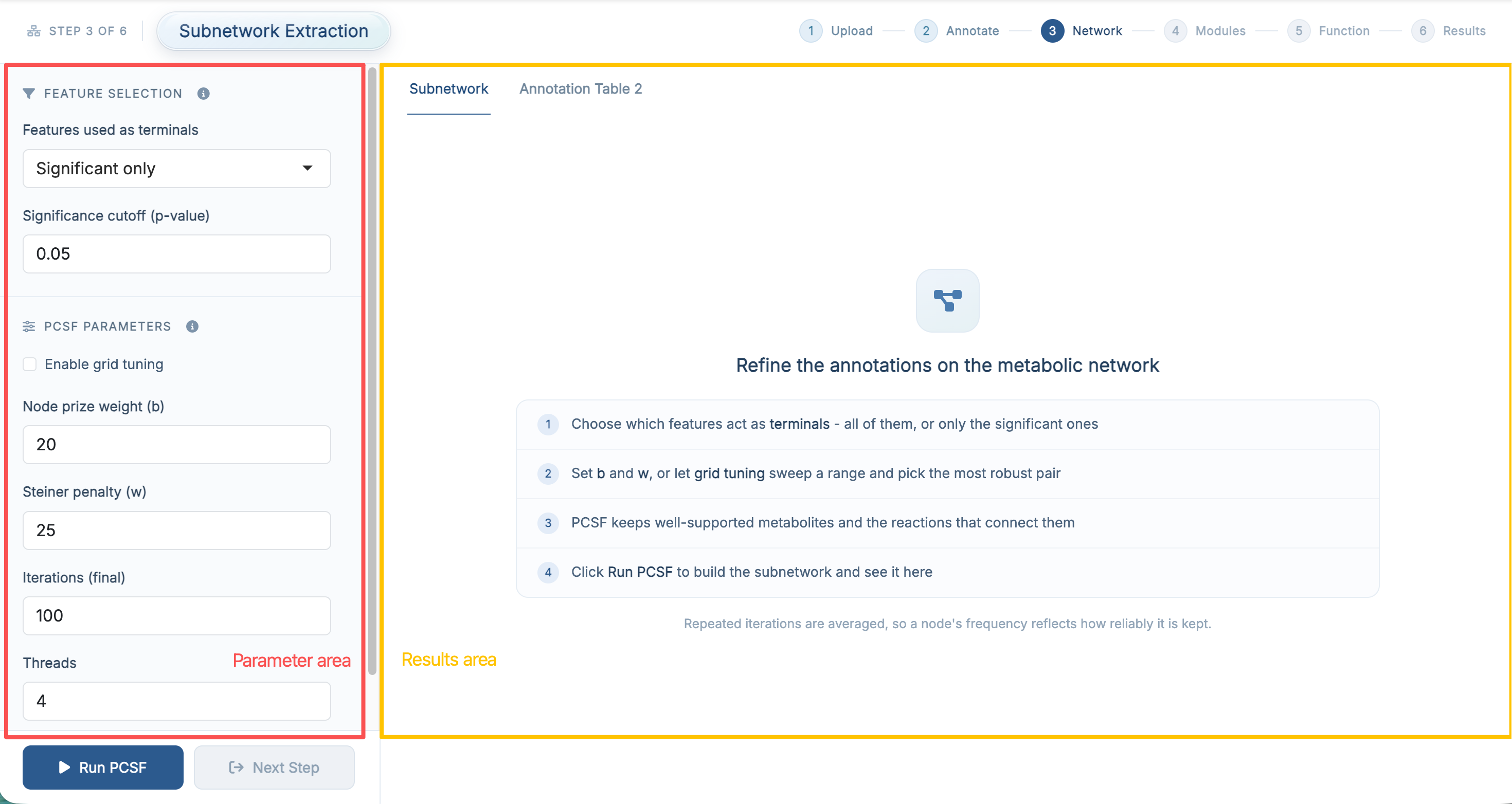
The purpose of this step is to use the PCSF strategy to extract a network-supported metabolite subnetwork for downstream module identification.
10.2 Parameter Area
| Section | Field | Default |
|---|---|---|
| Feature Selection | Features used as terminals (Significant only / All features) | Significant only |
| Significance cutoff (p-value), shown for Significant only | 0.05 |
|
| PCSF Parameters | Enable grid tuning | off |
| Node prize weight (b) | 20 |
|
| Steiner penalty (w) | 25 |
|
| Grid tuning range: b min / max / step, w min / max / step | 20 / 40 / 5 |
|
| Iterations (final) | 100 |
|
| Iterations (grid tuning) | 10 |
|
| Threads | 4 |
|
| Visualize PCSF subnetwork | on |
When Enable grid tuning is off, you set b and w directly; when it is on, those two fields are replaced by the grid ranges and by the tuning-iteration field. The meaning of each parameter is the same as in R package-Subnetwork Extraction.
If you are running the demo data for the first time, it is usually best to keep the default settings, leave grid tuning off, and run the step once before changing anything.
10.3 Run PCSF Subnetwork Extraction
Once the parameters are ready, click Run PCSF.
The app shows a progress card while the repeated PCSF runs are executed. When the step finishes successfully, the result panel on the right is updated automatically and the Next Step button becomes available.
If you enable grid tuning, the selected best b / w combination is recorded and shown later in the Analysis Parameters card on the Results Download page.
10.4 Result Area
10.4.1 Subnetwork
The Subnetwork tab shows the extracted PCSF network, provided Visualize PCSF subnetwork was enabled in the parameter area. If visualization is disabled, the run still finishes normally, but this tab stays empty.
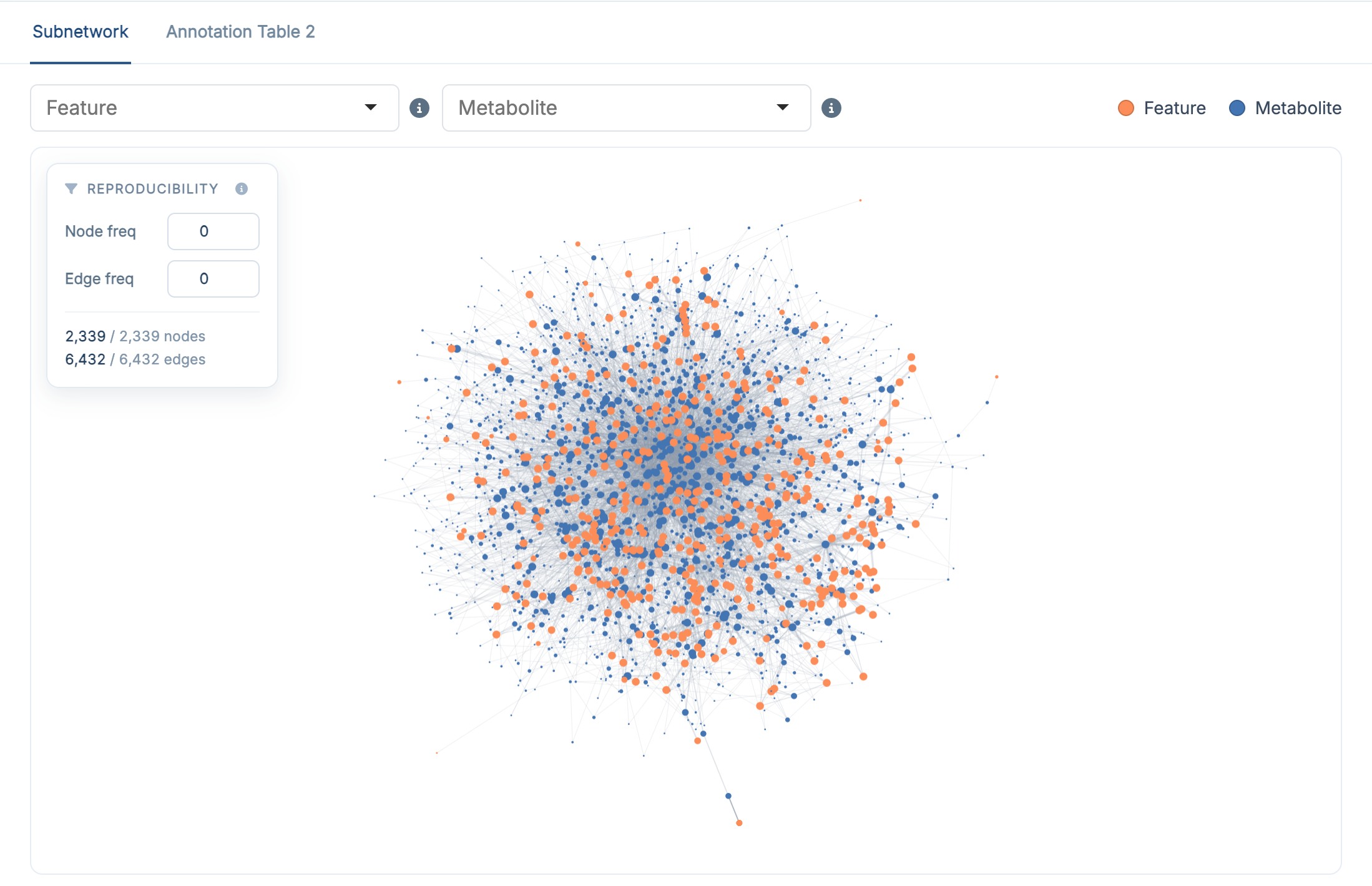
The network is interactive: you can zoom, drag and click nodes. Two selectors above the plot help you navigate a large network:
- the Feature selector highlights a chosen LC–MS feature and its directly connected metabolites
- the Metabolite selector highlights a chosen metabolite and its directly connected features
The rows listed under the network follow the current selection. The legend distinguishes Feature nodes (orange) from Metabolite nodes (blue).
10.4.2 Annotation Table 2
The Annotation Table 2 tab contains the network-refined annotation results generated after PCSF extraction, that is res$anno_feature_table2 in the R package. Compared with the previous annotation table, it adds the network evidence (edge_freq, weighted_anno_score, confidence_rank) and is the main output carried into the next step.
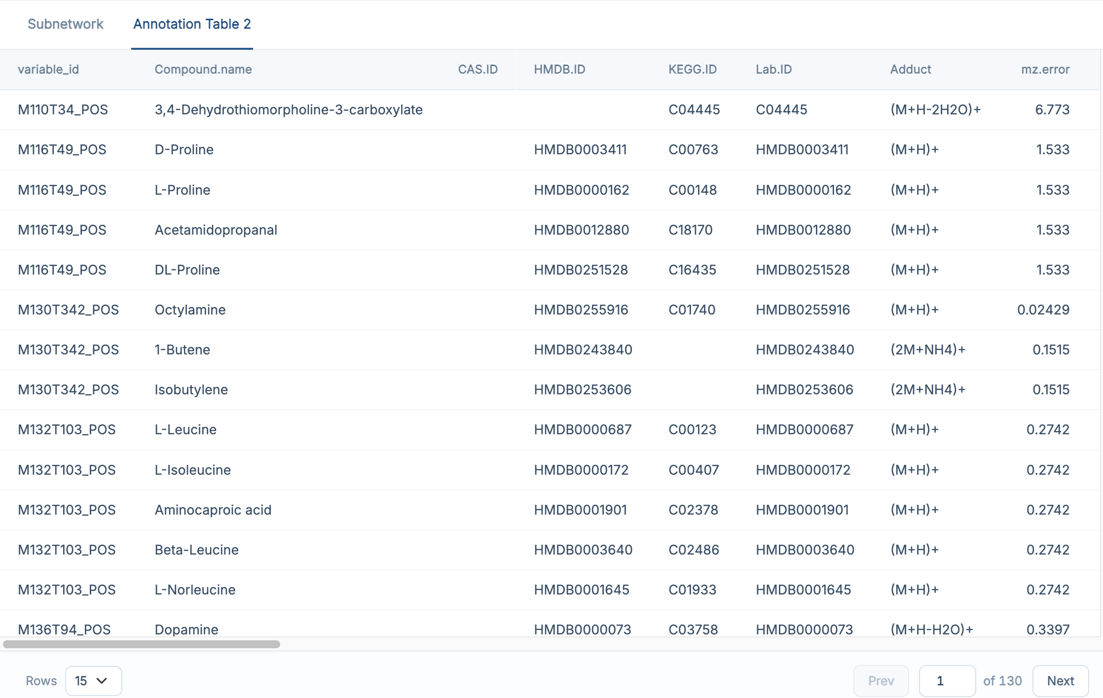
For a full explanation of the result columns, see R package-Subnetwork Extraction.
10.5 Recommended: Run the Demo Data First
If you followed the previous chapters and loaded the built-in demo data, the recommended workflow here is:
- keep the default parameter settings
- leave Enable grid tuning unchecked for the first run
- keep Visualize PCSF subnetwork enabled if you want to see the network directly
- click Run PCSF
- check the Subnetwork tab first
- then open Annotation Table 2 to inspect the refined results
This is the easiest way to understand what the PCSF step produces before tuning parameters on your own dataset.
If the result tab stays empty, first check whether Feature Annotation finished successfully in the previous step. Note that repeated PCSF runs are the slowest part of the workflow: lowering Iterations (final) gives a quicker first look, at the cost of robustness.
10.6 Next Step
Once subnetwork extraction is complete, click Next Step to continue to Module Identification.