Other tools for MS raw data processing

Xiaotao Shen (https://www.shenxt.info/)

true

Created on 2020-04-01 and updated on 2021-04-07

metflow2 also provide some useful tools for MS raw data processing.

---

Extract EICs from mzXML data

You can use metflow2 to extract peaks from the mzXML format data and then draw them.

Data preparation

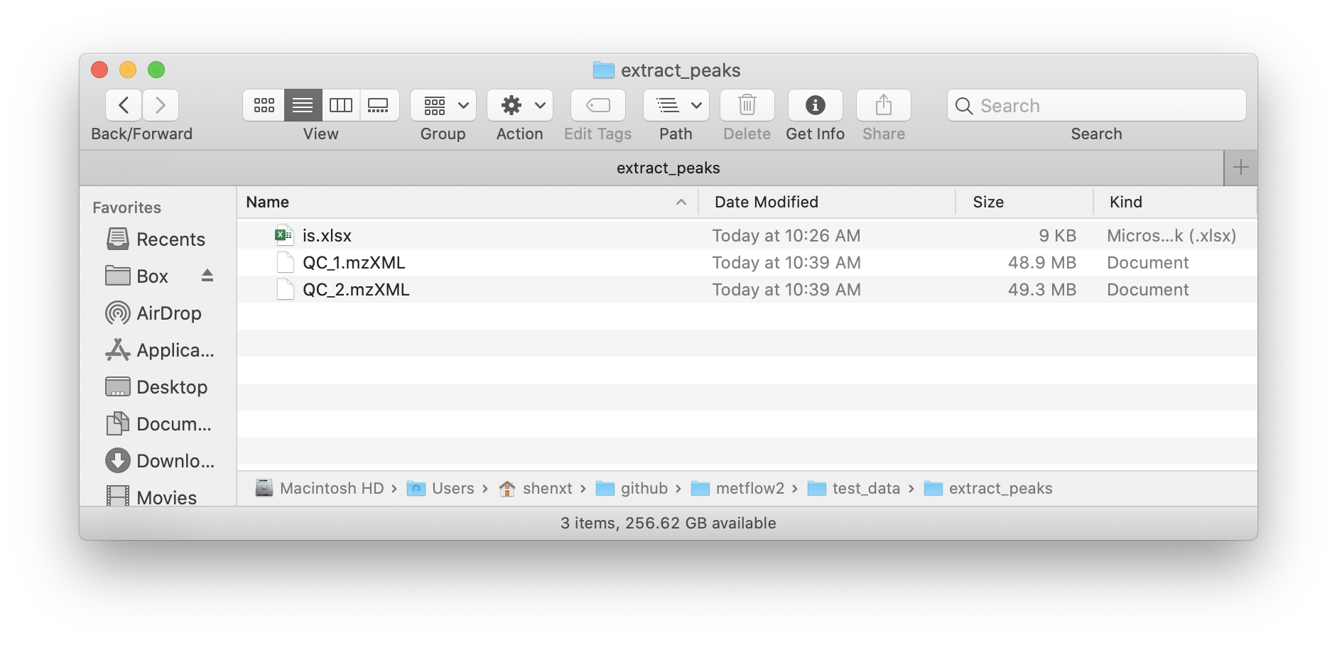
Put you mzXML data and the feature_table (xlsx format) in a folder and then set this folder as the working directory.

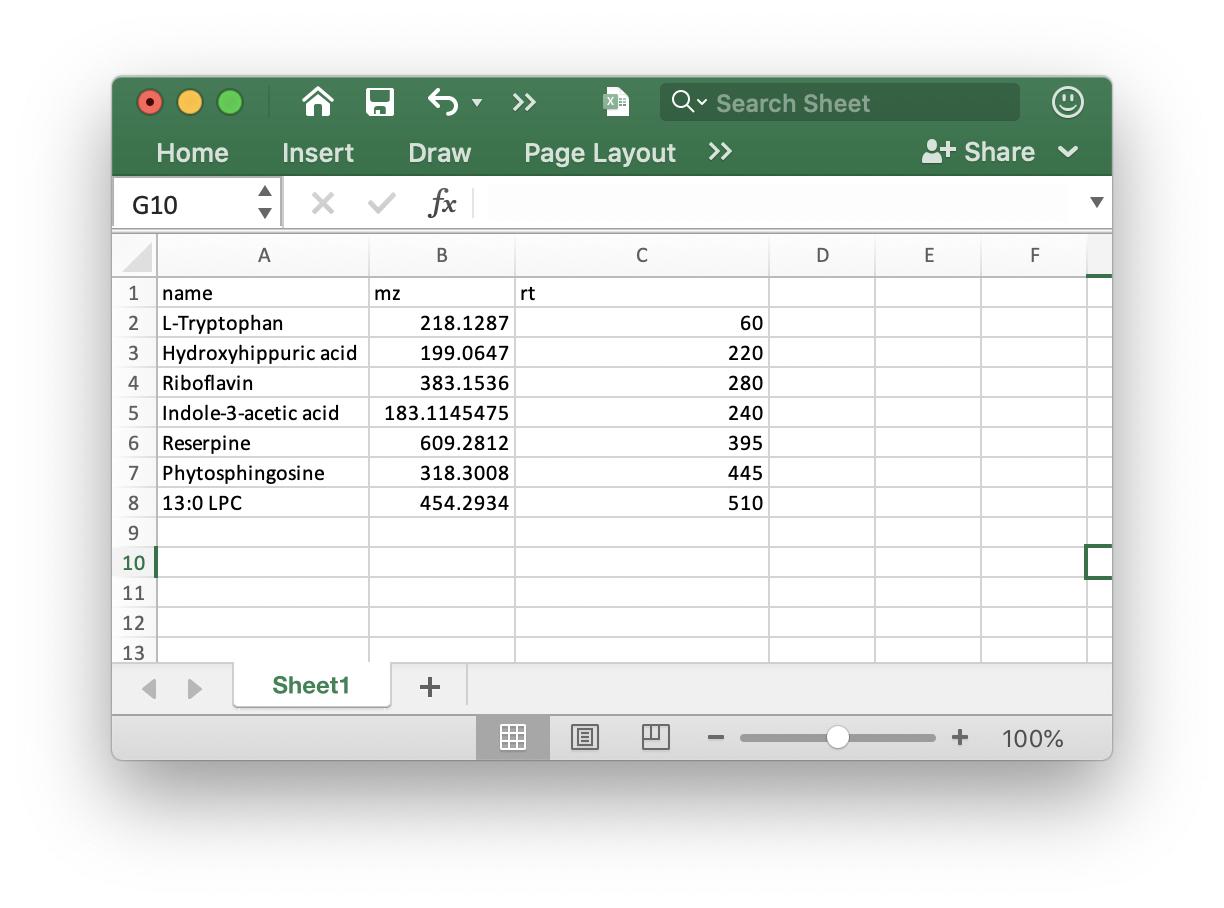
The feature_table should be xlsx format and like the below figure shows:

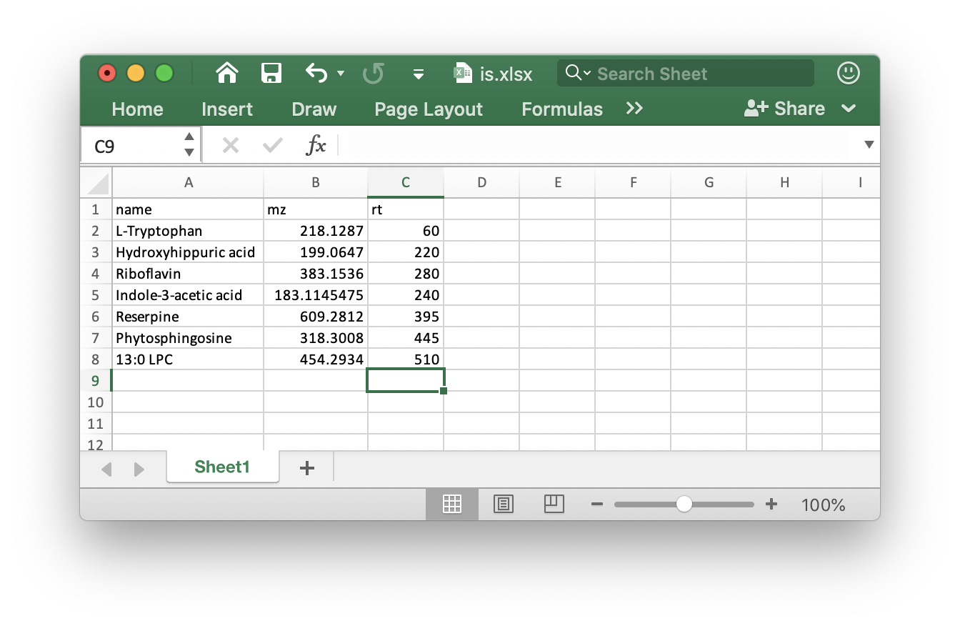
Note: The rt must in seconds.

We use the demo data from demoData package.

Load demo data

First we load the demo data from demoData package and then place them in a example folder.

library(demoData)
library(metflow2)
#> ✓ xcms    3.12.0     ✓ MSnbase 2.16.0
#> ✓ mzR     2.24.1
library(tidyverse)
#> ── Attaching packages ─────────────────────────────────────── tidyverse 1.3.0 ──
#> ✓ ggplot2 3.3.3     ✓ purrr   0.3.4
#> ✓ tibble  3.1.0     ✓ dplyr   1.0.4
#> ✓ tidyr   1.1.3     ✓ stringr 1.4.0
#> ✓ readr   1.4.0     ✓ forcats 0.5.0
#> ── Conflicts ────────────────────────────────────────── tidyverse_conflicts() ──
#> x dplyr::collect()    masks xcms::collect()
#> x dplyr::combine()    masks MSnbase::combine(), Biobase::combine(), BiocGenerics::combine()
#> x tidyr::expand()     masks S4Vectors::expand()
#> x dplyr::filter()     masks stats::filter()
#> x dplyr::first()      masks S4Vectors::first()
#> x dplyr::groups()     masks xcms::groups()
#> x dplyr::lag()        masks stats::lag()
#> x ggplot2::Position() masks BiocGenerics::Position(), base::Position()
#> x purrr::reduce()     masks MSnbase::reduce()
#> x dplyr::rename()     masks S4Vectors::rename()

##create a folder named as example
path <- file.path(".", "example")
dir.create(path = path, showWarnings = FALSE)

##get demo data
mzxml_data <- system.file("mzxml/POS/QC", package = "demoData")

file.copy(from = file.path(mzxml_data, dir(mzxml_data)), 
          to = path, overwrite = TRUE, 
          recursive = TRUE)

is_table <- system.file("mzxml/POS/", package = "demoData")

file.copy(from = file.path(is_table, "is.xlsx"), 
          to = path, overwrite = TRUE, 
          recursive = TRUE)

Now the demo mzXML data and feature table (is.xlsx)is in the ./example/ folder.

Extract peaks

Next, we use the extractPeaks() function for peak detection and alignment.

peak_data <- 
extractPeaks(
  path = path,
  ppm = 15,
  threads = 4,
  is.table = "is.xlsx",
  mz = NULL,
  rt = NULL,
  rt.tolerance = 40
)
#> Reading raw data, it will take a while...
#> Use old data.
#> ✔ OK
#> Extracting peaks, it will take a while...✔ OK

Some important arguments:

• ppm: Peak detection ppm.

• rt.tolerance: Peak detection ppm.

• is.table: If you add internal standards in your samples, you can provide the the is.table in the folder which your mzXML format data in. It must be xlsx format like the below figure shows:

Other parameters you can find here: processData().

Draw plots

After get the peak_data using extractPeaks() function, we can use show_peak() function to draw plot.

show_peak(object = peak_data, peak.index = 1)

If you don’t want to get the interactive plot, you can just set interactive as FALSE.

show_peak(object = peak_data, peak.index = 1, interactive = FALSE)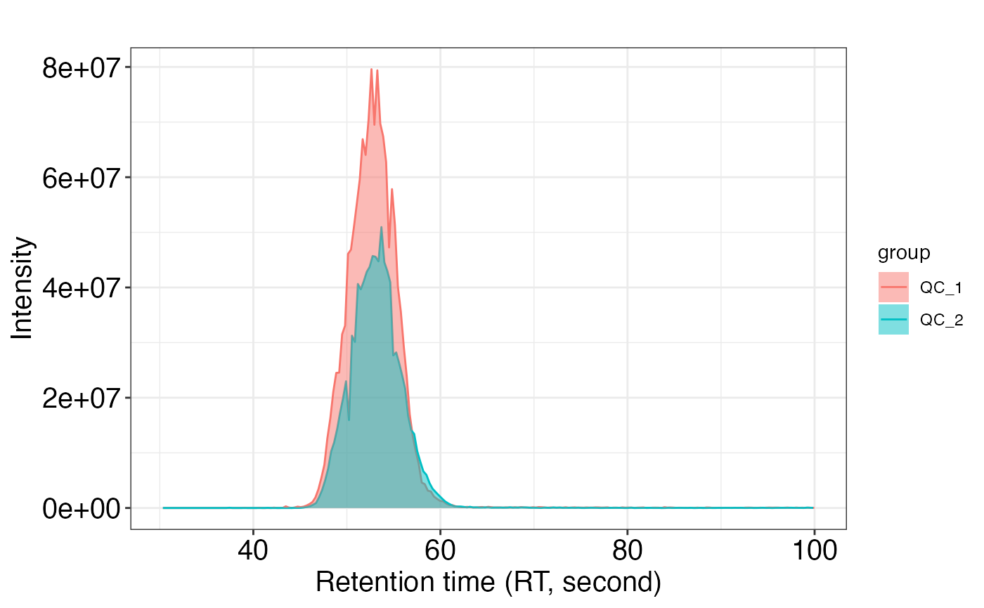

You can also set alpha as 0 to avoid the area color.

show_peak(object = peak_data, peak.index = 5, alpha = 0)